Unit 1: Exploring One-Variable Data - Summary Statistics
Measuring Center: The Typical Value
In AP Statistics, the goal of summarizing data is to simplify a complex set of numbers into values that describe the distribution's key features. The first feature we look for is the center—a single number that represents the "typical" value of the dataset.
The Mean (Arithmetic Average)
The mean is the arithmetic average of a distribution. Because it takes the specific value of every observation into account, it is the fundamental balancing point of the distribution (like a fulcrum on a seesaw).
Notation:
- Sample Mean: $\bar{x}$ (pronounced "x-bar")
- Population Mean: $\mu$ (the Greek letter "mu")
Formula:
For a sample of size $n$ with observations $x1, x2, …, x_n$:
Where $\sum$ (sigma) means "sum of."
The Median (Midpoint)
The median is the midpoint of the distribution. It is the value such that half the observations are smaller and half are larger. To find the location of the median in an ordered list of $n$ numbers, calculate $\frac{n+1}{2}$.
- If $n$ is odd, the median is the value at the exact center.
- If $n$ is even, the median is the average of the two center observations.
Robustness (Resistance) and Skewness
A critical concept in Unit 1 is understanding how extreme values (outliers) affect these measures.
- Non-Resistant (Non-Robust): The Mean is sensitive to extreme values. One massive outlier pulls the mean toward it.
- Resistant (Robust): The Median is resistant to extreme values. A billionaire walking into a room of teachers changes the mean income drastically but barely touches the median income.
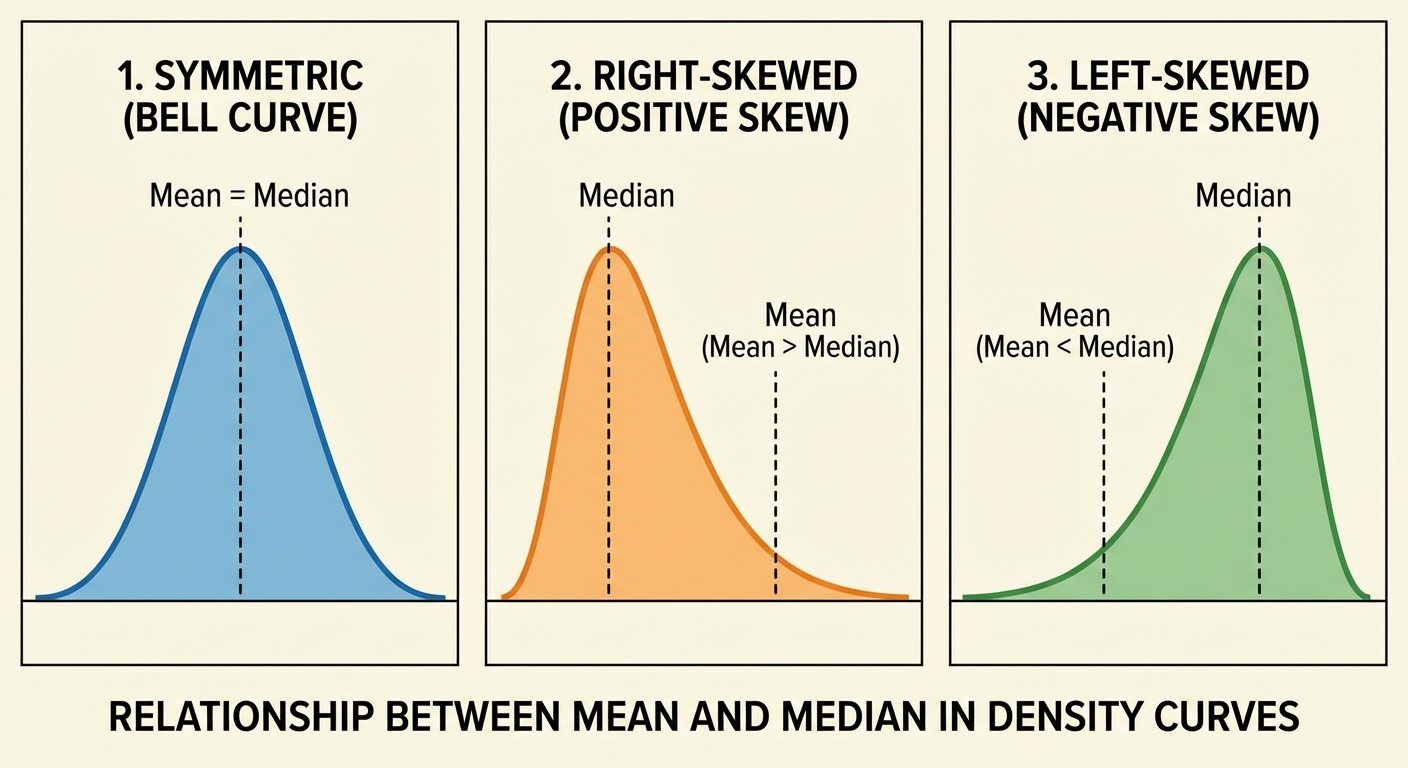
Relationship between Shape and Center:
| Distribution Shape | Relationship |
|---|---|
| Symmetric | $\text{Mean} \approx \text{Median}$ |
| Skewed Right (Tail right) | $\text{Mean} > \text{Median}$ |
| Skewed Left (Tail left) | $\text{Mean} < \text{Median}$ |
Measuring Variability: The Spread
Describing the center is not enough; we must also describe how spread out the data is. Is the data consistent (low variability) or volatile (high variability)?
The Range
The most basic measure of spread. It is a single number, not an interval.
- Note: Like the mean, the Range is non-resistant. A single outlier increases the range significantly.
The Interquartile Range (IQR)
The IQR measures the range of the middle 50% of the data. Because it ignores the upper and lower 25% of data points (which is where outliers live), the IQR is a resistant measure of spread.
- $Q_1$ (First Quartile): The median of the lower half of the data.
- $Q_3$ (Third Quartile): The median of the upper half of the data.
Standard Deviation and Variance
The standard deviation is the most common measure of spread when using the mean as the center. It measures the typical distance of the values from the mean.
Formulas:
Variance ($s^2_x$): The average squared distance from the mean.
Standard Deviation ($s_x$): The square root of the variance (returns the unit to the original scale).
Why divide by $n-1$?
Dividing by $n-1$ (degrees of freedom) instead of $n$ creates an unbiased estimator. It corrects for the fact that sample spread tends to consistently underestimate the true population spread.
Properties of Standard Deviation:
- $s_x \ge 0$. It is only 0 if all numbers in the dataset are identical.
- Ideally used for symmetric distributions.
- Non-resistant. Outliers squared create massive contributions to variance, inflating the standard deviation.
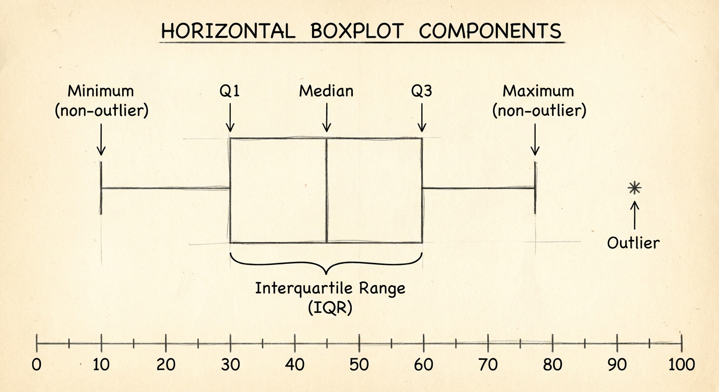
Boxplots and the Five-Number Summary
The Five-Number Summary
This summary divides the dataset into four equal parts (quartiles), each containing 25% of the data.
- Minimum
- First Quartile ($Q_1$)
- Median
- Third Quartile ($Q_3$)
- Maximum
The 1.5 $\times$ IQR Rule for Outliers
In AP Statistics, you cannot simply say a point "looks" like an outlier. You must justify it mathematically.
Outlier Boundaries (Fences):
- Lower Fence: $Q_1 - 1.5(IQR)$
- Upper Fence: $Q_3 + 1.5(IQR)$
Any data point falling outside these fences is considered an outlier.
Boxplots (Box-and-Whisker Plots)
A boxplot is the graphical representation of the five-number summary.
- The Box spans from $Q1$ to $Q3$ (the IQR).
- The line inside the box is the Median.
- The Whiskers extend to the lowest and highest observations that are not outliers.
- Outliers represent individual dots beyond the whiskers.
Worked Example
Dataset: $2, 4, 5, 6, 7, 9, 20$
Calculate Stats:
- $n = 7$
- Median: 6 (4th number)
- $Q_1$: 4 (Median of lower half $2, 4, 5$)
- $Q_3$: 9 (Median of upper half $7, 9, 20$)
- $IQR = 9 - 4 = 5$
Check for Outliers:
- Lower Limit: $4 - 1.5(5) = -3.5$. No values below -3.5.
- Upper Limit: $9 + 1.5(5) = 16.5$. The value 20 is above 16.5.
Conclusion: 20 is a mathematical outlier. The whisker on the right would stop at 9, and 20 would be a distinct point.
Summary: Choosing the Right Statistics
In the AP exam, you are often asked to compare distributions. Your choice of summary statistics depends entirely on the shape of the data.
| Distribution Shape | Measure of Center | Measure of Spread |
|---|---|---|
| Symmetric / Normal | Mean ($\bar{x}$) | Standard Deviation ($s_x$) |
| Skewed / Has Outliers | Median | IQR |
Why? Because Mean and SD are sensitive to skew/outliers, while Median and IQR are resistant.
Common Mistakes & Pitfalls
Confusing Statistic vs. Parameter:
- Remember: Statistics come from Samples ($\bar{x}, s$). Parameters come from Populations ($\mu, \sigma$).
Misinterpreting the Standard Deviation:
- Bad answer: "The standard deviation is 5.2."
- Good answer: "The values in this sample typically vary by about 5.2 units from the mean."
- Don't forget the context and units!
Incorrect Boxplot Whiskers:
- Students often draw whiskers to the "fences" calculated by the 1.5 IQR rule. This is wrong. Whiskers go to the last actual data point inside the fence.
Vague Comparisons:
- When comparing two distributions, never just list the stats (e.g., "Dataset A has mean 5, Dataset B has mean 10"). You must use comparative language: "The center of Dataset B (10) is higher than the center of Dataset A (5)."
Mnemonic: CUSS and BS
When asked to describe or compare distributions, remember to address:
- Center (Mean/Median)
- Unusual Features (Outliers/Gaps)
- Shape (Skewness/Modes)
- Spread (Range/SD/IQR)
- Be Specific (Always include context/units!)