AP Statistics Unit 9: Inference for Slope
Introducing Statistics for the Slope of a Regression Model
In previous units, you learned how to calculate the Least Squares Regression Line (LSRL) to describe the relationship between two quantitative variables in a sample. The equation was $\hat{y} = b0 + b1x$ (or $\hat{y} = a + bx$).
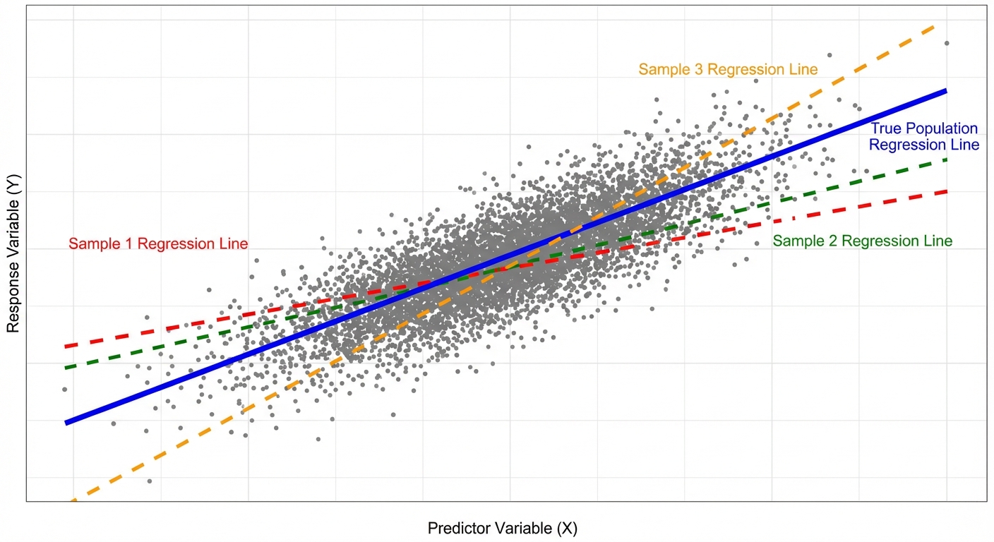
However, in Unit 9, we shift from description to inference. We acknowledge that our sample data is just a small slice of a larger population. If we took a different random sample, we would get a slightly different regression line. We use inference to determine if the linear relationship we see in our sample actually exists in the population.
Population vs. Sample Notation
It is vital to distinguish between the statistics calculated from data and the parameters they estimate.
| Concept | Population Parameter (True value) | Sample Statistic (Estimate) |
|---|---|---|
| y-intercept | $\alpha$ or $\beta_0$ | $a$ or $b_0$ |
| Slope | $\beta$ or $\beta_1$ | $b$ or $b_1$ |
The True Regression Model:
We assume the true relationship in the population takes the form:
Where $\epsilon$ represents the random error (residuals) that are normally distributed.
The Sampling Distribution of $b$
If you took many random samples of the same size $n$ from the population and calculated the slope ($b$) for each, the distribution of those slopes would be:
- Centered at the true population slope $\beta$ (it is an unbiased estimator).
- Normally distributed (provided the conditions below are met).
- Have a standard deviation (standard error) that decreases as the sample size $n$ increases or as the spread of $x$-values increases.
Conditions for Inference (LINER)
Before performing a test or creating an interval for a regression slope, you must define the LINER conditions. If these are violated, your inference may be invalid.
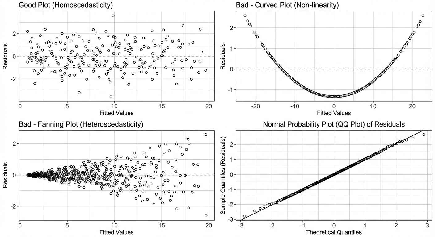
- L — Linear: The relationship between $x$ and $y$ is linear. Check this by looking at the scatterplot (should look straight) and the residual plot (should show no curved pattern).
- I — Independent: Individual observations are independent. If sampling without replacement, the population must be at least $10\times$ the sample size ($10\%$ condition).
- N — Normal: The responses ($y$) vary normally around the true regression line. Check this by looking at a histogram or Normal Probability Plot of the residuals (should show no strong skew/outliers).
- E — Equal Variance (Homoscedasticity): The standard deviation of $y$ is the same for all values of $x$. Check the residual plot — the "fuzz" or vertical spread of dots should be roughly consistent across the graph (no "fan" shapes).
- R — Random: The data comes from a random sample or a randomized experiment.
Confidence Interval for the Slope of a Regression Model
A confidence interval allows us to estimate the true slope $\beta$ of the population regression line.
The Formula
Where:
- $b$: The sample slope estimate.
- $t^*$: The critical value based on the confidence level and Degrees of Freedom.
- $SEb$: The Standard Error of the slope. (Note: calculating $SEb$ by hand is tedious and rarely required on the AP exam; it is almost always provided in a computer output table).
Degrees of Freedom ($df$):
Why $n-2$? We estimate two parameters ($b0$ and $b1$) to fit the line usually, which costs us two degrees of freedom.
Reading Computer Output
Most AP Statistics questions on this topic provide a regression table. You must know where to look.
| Predictor (Term) | Coef | SE Coef | T-Value | P-Value |
|---|---|---|---|---|
| Constant (Intercept) | $14.5$ | $2.1$ | $6.90$ | $0.000$ |
| Hours Study (Slope) | $3.2$ | $0.45$ | $7.11$ | $0.000$ |
In this table:
- $b = 3.2$
- $SE_b = 0.45$
Worked Example: Confidence Interval
Scenario: A teacher wants to estimate the true slope of the relationship between hours studied ($x$) and test score ($y$). A sample of $n=20$ students yields $b=3.2$ and standard error of slope $SE_b = 0.45$. Construct a 95% confidence interval.
Step 1: Identify
We need a 95% CI for the population slope $\beta$.
Step 2: Conditions
(Assume LINER conditions are met for this example).
Step 3: Calculate
- $df = 20 - 2 = 18$.
- Using a t-table or calculator (
invT(0.975, 18)), $t^* \approx 2.101$. - Formula: $3.2 \pm 2.101(0.45)$
- $3.2 \pm 0.945$
- Interval: $(2.255, 4.145)$
Step 4: Conclude
We are 95% confident that the interval from 2.255 to 4.145 captures the true slope of the relationship between hours studied and test scores. (Wait—always add context!) For every additional hour studied, the test score increases by between 2.26 and 4.15 points on average in the population.
Significance Test for the Slope of a Regression Model
Usually, we want to know if there is any useable linear relationship at all. If the true slope $\beta = 0$, then $x$ is useless for predicting $y$ linearly (the line is horizontal).
Hypotheses
- Null Hypothesis ($H_0$): $\beta = 0$ (There is no linear relationship between $x$ and $y$).
- Alternative Hypothesis ($H_a$):
- $\beta \neq 0$ (There is a linear relationship).
- $\beta > 0$ (There is a positive linear relationship).
- $\beta < 0$ (There is a negative linear relationship).
Test Statistic Formula
Since we almost always assume $\beta0 = 0$ in the null hypothesis:
- Degrees of Freedom: $df = n - 2$
Using Computer Output for Tests
Referencing the table in the previous section:
- T-Value: The computer usually calculates the T-statistic for the two-sided test ($H_a: \beta \neq 0$) automatically. In the table, $T = \frac{3.2}{0.45} \approx 7.11$.
- P-Value: The P-value listed (0.000) represents the probability of getting a sample slope this far from 0 if there really were no relationship.
Worked Example: Hypothesis Test
Scenario: Using the same data ($n=20$, $t=7.11$). Is there convincing evidence of a positive linear association?
Hypotheses:
- $H_0: \beta = 0$
- $H_a: \beta > 0$
Calculate:
- $t = 7.11$
- $df = 18$
- $P\text{-value} = \text{tcdf}(7.11, \infty, 18) \approx 0.0000002$
Conclusion:
- Since $P < 0.05$, we reject $H_0$.
- There is convincing evidence that there is a positive linear relationship between hours studied and test scores.
Common Mistakes & Exam Tips
1. Confusing Extrapolation with Inference
Inference tells you if a relationship likely exists in the population. It does not authorize you to predict values far outside the domain of $x$ (extrapolation), even if the P-value is very low.
2. The "Intercept" Trap
Computer outputs list specific rows for "Constant" (intercept) and the variable name (slope). Students often grab the wrong numbers. Always look for the row with the variable name (e.g., "Hours Study") to find slope data. The "Constant" row is rarely tested in inference.
3. Forgetting Degrees of Freedom
In simple linear regression, $df = n - 2$. Students often simply use $n$ or $n-1$, which leads to slightly incorrect critical values and P-values.
4. Interpreting the Interval Incorrectly
Wrong: "We are 95% confident that the slope is 3.2."
Right: "We are 95% confident that the true population slope falls between X and Y."
Also, ensure your context explains the rate of change (change in $y$ for every 1 unit of $x$).
5. Interpreting "Zero" in the Interval
If your Confidence Interval for the slope includes 0 (e.g., $[-0.5, 2.3]$), you cannot reject the null hypothesis at the corresponding alpha level. It suggests there is no convincing evidence of a linear relationship.