Mastering Categorical Data Inference: Proportions
Unit 6: Inference for Categorical Data: Proportions
This unit focuses on making conclusions (inferences) about population proportions based on sample data. We will cover Confidence Intervals (estimating a parameter) and Significance Tests (assessing a claim) for both single populations and the difference between two populations.
The core logic relies on the sampling distributions discussed in Unit 5. Specifically, because sample proportions vary (sampling variability), we use probability to quantify the uncertainty of our estimates.
The Logic of Confidence Intervals
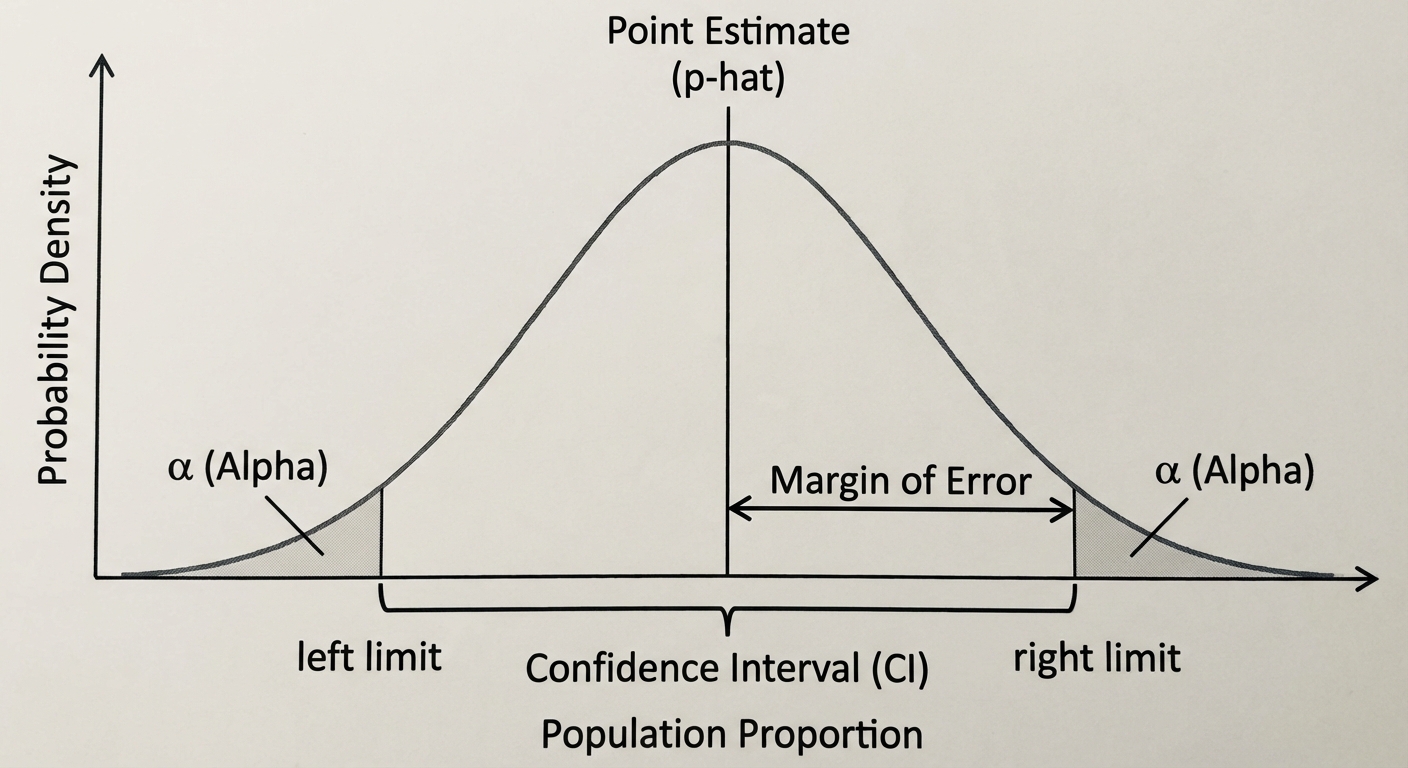
A Confidence Interval is a range of plausible values for an unknown population parameter (such as a proportion $p$). It is constructed from sample data.
confidence Level vs. Confidence Interval
Students often confuse these two concepts. It is vital to distinguish them:
- Confidence Interval (The Result): The calculated range (e.g., $0.45$ to $0.55$). We interpret this by saying: "We are 95% confident that the interval from 0.45 to 0.55 captures the true population proportion $p$."
- Confidence Level (The Method's Success Rate): This describes the procedure. If we were to take many, many samples of the same size from the same population and construct a confidence interval from each, about C% (e.g., 95%) of those intervals would successfully capture the true population parameter.
The Anatomy of an Interval
Most confidence intervals follow this structure:
- Statistic (Point Estimate): The value from your sample (e.g., $\hat{p}$). It is your best guess.
- Margin of Error (ME): Everything to the right of the $\pm$. It reflects the precision of the estimate. $ \text{ME} = ( ext{Critical Value}) \times ( ext{Standard Error})$.
Conditions for Inference
Before calculating intervals or tests, you must verify three conditions to ensure the math models (Normal/z-procedures) are invalid.
1. Random (Independence Assumption)
- Why? To ensure the sample is representative and to minimize bias.
- How to Check: The problem must state the data comes from a Simple Random Sample (SRS) or a randomized experiment.
2. 10% Condition (Independence)
- Why? Sampling is usually done without replacement. If we sample too much of the population, observations aren't independent (probability changes). The formula for standard deviation assumes independence.
- How to Check: Verify that the population size ($N$) is at least 10 times the sample size ($n$).
3. Large Counts (Normality Assumption)
- Why? To use the Normal Approximation ($z$-scores), the sampling distribution of $\hat{p}$ must be approximately Normal.
- How to Check: The expected number of successes and failures must both be at least 10.
- For One-Sample Intervals: $n\hat{p} \ge 10$ and $n(1-\hat{p}) \ge 10$.
- For One-Sample Tests: $np0 \ge 10$ and $n(1-p0) \ge 10$ (use the null/hypothesized $p$).
Example 6.1 (Checking Conditions)
Scenario: A researcher picks an SRS of size $n=80$ from a large population to estimate a proportion. Which population proportion $p$ would verify the Normality condition?
- Options: (A) 0.10, (B) 0.15, (C) 0.99
Solution: We need expected successes ($np$) and failures ($nq$ or $n(1-p)$) $\ge 10$.
- (A) $80(0.10) = 8$. (Fail, $<10$)
- (C) $80(0.99) = 79.2$ (Success check ok), but failures $80(0.01) = 0.8$. (Fail, $<10$)
- (B) $np = 80(0.15) = 12$ and $n(1-p) = 80(0.85) = 68$. Both are $\ge 10$. This is valid.
One-Sample Confidence Interval for $p$
When estimated standard deviation is calculated from sample data, it is called Standard Error (SE). For a sample proportion $\hat{p}$, the standard error is:
The Confidence Interval Formula:
- $z^*$ (Critical Value): Determined by the confidence level. Common values:
- 90% $\rightarrow z^* = 1.645$
- 95% $\rightarrow z^* = 1.960$
- 99% $\rightarrow z^* = 2.576$
Example 6.2: First Date Etiquette
Problem: In an SRS of 550 young adults, 42% ($\,\hat{p}=0.42$) believe the person who asks for the date should pay. Construct a 99% confidence interval for the true proportion.
Step 1: State
We want to estimate $p$, the true proportion of all young adults who believe the asker should pay, with 99% confidence.
Step 2: Plan
- Method: One-sample $z$-interval for $p$.
- Random: Stated SRS.
- 10% Condition: It is reasonable to assume there are more than $550 \times 10 = 5,500$ young adults.
- Large Counts: $550(0.42) = 231$ and $550(0.58) = 319$. Both $\ge 10$.
Step 3: Do
Interval: $(0.366, 0.474)$
Step 4: Conclude
We are 99% confident that the true proportion of young adults who believe the asker should pay is between 36.6% and 47.4%.
Claim Verification: Does this support the claim that fewer than 50% hold this belief?
Answer: Yes. Because the entire interval (0.366 to 0.474) is strictly below 0.50, we have convincing evidence.
Significance Tests for a Proportion
A significance test asks: "Is the difference between my sample and the claim just random chance, or is the claim wrong?"
The Hypotheses
- Null Hypothesis ($H0$): A statement of "no difference" or equality. $H0: p = p0$ (where $p0$ is the claimed value).
- Alternative Hypothesis ($H_a$): What we suspect is actually true.
- $Ha: p < p0$ (Left-tailed)
- $Ha: p > p0$ (Right-tailed)
- $Ha: p \neq p0$ (Two-tailed)
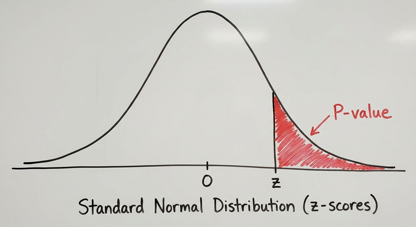
The Test Statistic ($z$)
Since we assume $H0$ is true, we use $p0$ (the null parameter) for the standard deviation, NOT the sample $\hat{p}$.
Example 6.3: Union Strike
Problem: A union claims 75% support for a strike ($p_0=0.75$). Management believes support is lower. In a random sample of 125 members, 87 said they would strike. Test at $\alpha=0.05$.
1. State: $H0: p = 0.75$ vs $Ha: p < 0.75$. $\alpha = 0.05$.
2. Plan: One-sample $z$-test.
- Checks: $125(0.75)=93.75$ and $125(0.25)=31.25$. Random = Yes. 10% = Yes.
3. Do:
Sample proportion $\hat{p} = 87/125 = 0.696$.
Using a calculator or table: P-value $\approx 0.082$.
4. Conclude:
Since $P\text{-value} (0.082) > \alpha (0.05)$, we fail to reject $H_0$. There is insufficient evidence to conclude that support for the strike is less than 75%.
Errors and Power in Testing
When we make a conclusion, we might be wrong. There are two specific types of errors.
Type I and Type II Errors
| $H_0$ is actually True | $H_0$ is actually False | |
|---|---|---|
| Reject $H_0$ | Type I Error (False Positive) Prob = $\alpha$ (Significance Level) | Correct Decision Prob = Power |
| Fail to Reject $H_0$ | Correct Decision Prob = $1 - \alpha$ | Type II Error (False Negative) Prob = $\beta$ |
- Type I Error ($\,\alpha$): Rejecting a true null. (Example: The union strikes thinking they have support, but they actually don't).
- Type II Error ($\,\beta$): Failing to reject a false null. (Example: The union does not strike thinking they lack support, when they actually have it).
- Power ($1 - \beta$): The probability of correctly rejecting a false null hypothesis.
Increasing Power
You can increase the Power of a test by:
- Increasing sample size ($n$): Reduces variability, making it easier to detect a difference.
- Increasing $\alpha$: Makes it easier to reject $H_0$ (but increases Type I error risk).
- Larger Effect Size: If the true parameter is very far from the null, it's easier to detect.
Inference for the Difference of Two Proportions
We often compare two groups (e.g., "Do nurses on night shifts have lower satisfaction than day shifts?").
Notation
- Population 1: $p1$, Sample 1: $\hat{p}1$, Size: $n_1$
- Population 2: $p2$, Sample 2: $\hat{p}2$, Size: $n_2$
Two-Sample Confidence Interval
We estimate the difference: $p1 - p2$.
Standard Error (Unpooled):
When making an interval, we do not assume the proportions are equal, so we keep them separate.
Formula:
Example 6.4: Nurse Satisfaction
- Shift 1 (Day): $n1=125, \hat{p}1 = 0.84$
- Shift 2 (Night): $n2=150, \hat{p}2 = 0.72$
- Goal: 90% Confidence Interval for difference (Day - Night).
Do Step:
Difference = $0.84 - 0.72 = 0.12$. Critical value ($z^*$ for 90%) = 1.645.
Interpretation: We are 90% confident the interval 0.039 to 0.201 captures the true difference. Since the interval is entirely positive, we have evidence that Day shift satisfaction is higher.
Two-Sample Significance Test
The Null Hypothesis
Usually, we test if there is no difference.
Pooling: The Critical Distinction
Because $H0$ assumes $p1 = p2$, we assume both samples come from the same population with a single common proportion. We must combine (pool) the data to get the best estimate of this common proportion, $\hat{p}c$.
Test Statistic Formula (Pooled):
Example 6.5: Child Welfare
- First Nations: $n1=1500, X1=162$. $\hat{p}_1 \approx 0.108$.
- Non-Aboriginal: $n2=1600, X2=23$. $\hat{p}_2 \approx 0.014$.
- Test $H0: p1 = p2$ vs $Ha: p1 > p2$ (Is proportion higher for First Nations?).
Pooling:
Calculate z:
Conclusion: $P \approx 0$. Reject $H_0$. Strong evidence that the proportion is higher for First Nations children.
Common Mistakes & Pitfalls
Pooling Incorrectly:
- NEVER pool for Confidence Intervals (we don't assume $p1=p2$).
- ALWAYS pool for Hypothesis Tests when $H0: p1 = p_2$.
Standard Error vs. Standard Deviation:
- In One-Sample Tests, use the null parameter $p0$ inside the square root: $\sqrt{p0(1-p_0)/n}$.
- In One-Sample Intervals, use the sample statistic $\hat{p}$: $\sqrt{\hat{p}(1-\hat{p})/n}$.
Accepting the Null:
- Never write "We accept $H0$." Always write "We fail to reject $H0$." (Lack of evidence for the alternative $\neq$ proof of the null).
Phrasing the Conclusion:
- Always link the P-value to $\alpha$ explicitly: "Since $P < \alpha$, we reject…"
- Always state the conclusion in context of the alternative hypothesis: "We have convincing evidence that [context of $H_a$]."