AP Statistics: Unit 5 - Sampling Distributions
Introduction to Sampling Distributions
Fundamentals of Sampling Distributions
Parameter vs. Statistic
In statistics, it is crucial to distinguish between the numbers that describe a whole population and the numbers that describe a sample drawn from that population.
- Parameter: A number that describes some characteristic of the population. In statistical practice, the value of a parameter is usually unknown.
- Notation: $\mu$ (population mean), $p$ (population proportion), $\sigma$ (population standard deviation).
- Statistic: A number that describes some characteristic of a sample. The value of a statistic can be computed directly from the sample data. We use statistics to estimate parameters.
- Notation: $\bar{x}$ (sample mean), $\hat{p}$ (sample proportion), $s$ (sample standard deviation).
What is a Sampling Distribution?
If we take repeated random samples of the same size $n$ from the same population, the value of the statistic (like the mean $\bar{x}$ or proportion $\hat{p}$) will vary from sample to sample. This concept is typically visualized as:
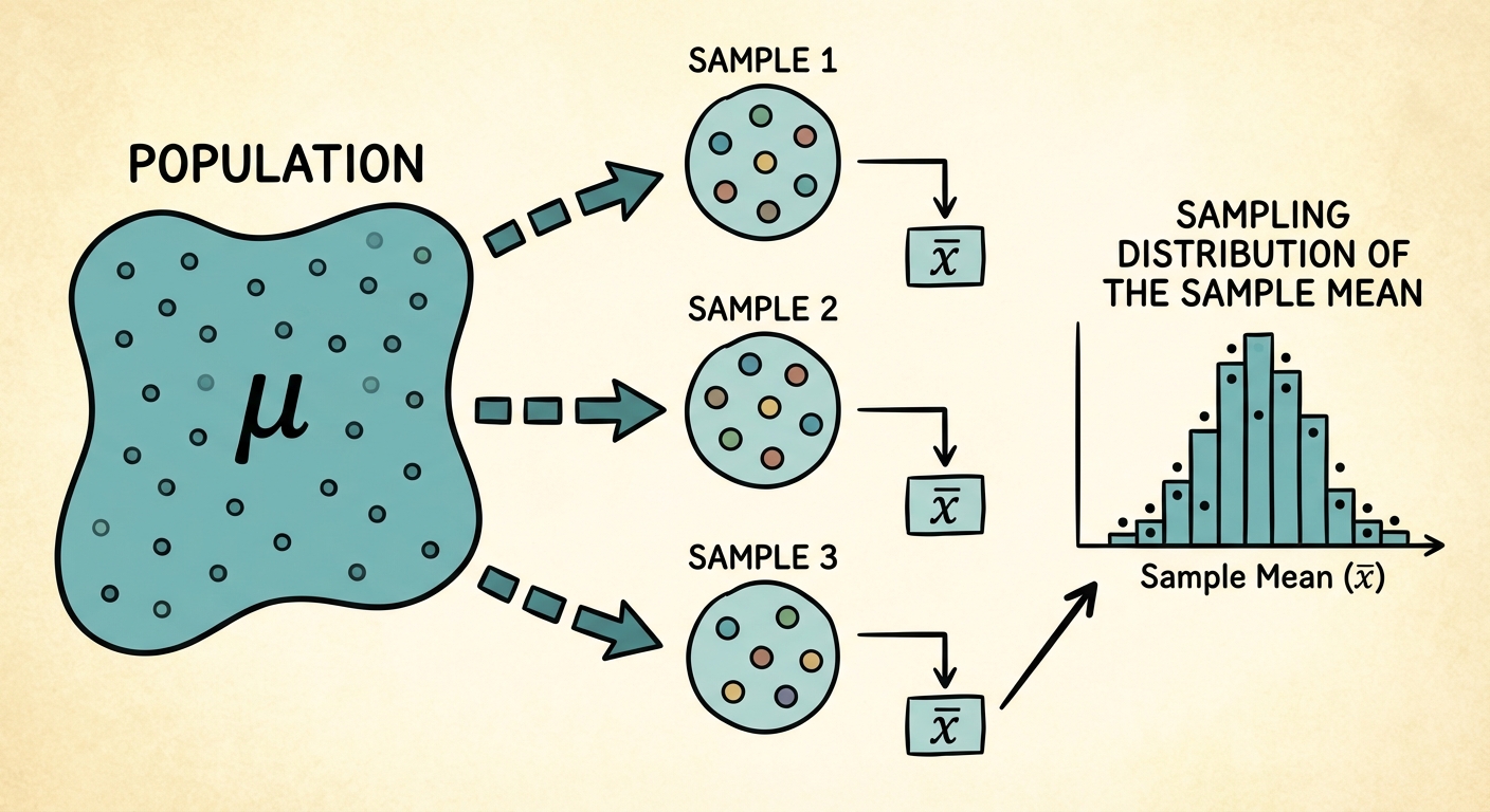
Definition: The sampling distribution of a statistic is the distribution of values taken by the statistic in all possible samples of the same size from the same population.
Bias and Variability
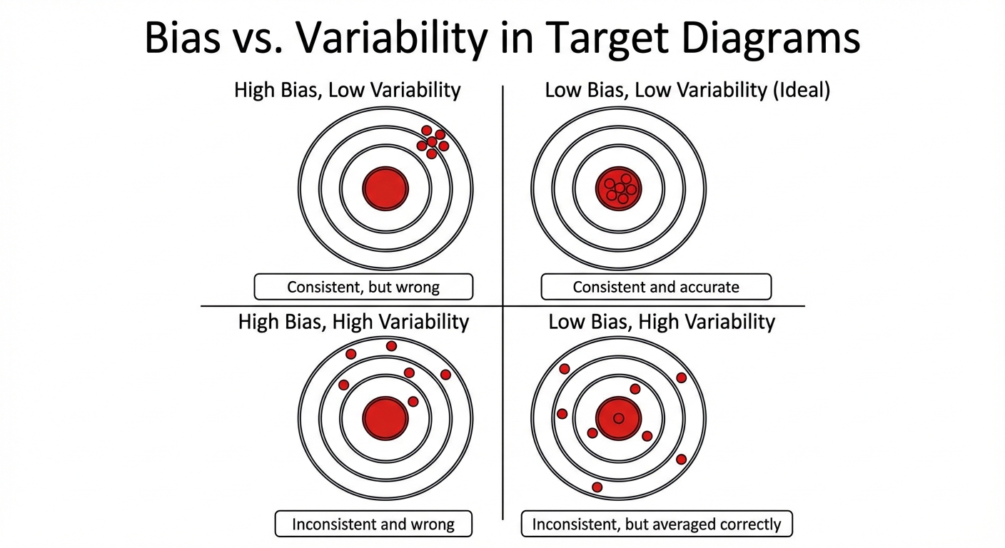
When evaluating a statistic as an estimator of a parameter, we look at twomain characteristics: bias (center) and variability (spread).
Biased vs. Unbiased Estimators
- Unbiased Estimator: A statistic is unbiased if the mean of its sampling distribution is equal to the true value of the parameter being estimated.
- $\hat{p}$ and $\bar{x}$ are unbiased estimators of $p$ and $\mu$, respectively.
- Bias: Failure of the sampling distribution to center on the population parameter.
Variability
- Variability: Describes how spread out the values of the sample statistic are.
- Larger samples ($n$) result in smaller variability. This is a key rule: Averages based on larger samples vary less than averages based on smaller samples.
➥ Example 5.1: Analyzing Estimators
Imagine manufacturing baseballs with a target weight of 146g. You test different estimators (A, B, C, D) using various sample sizes.
- Unbiased: If the estimator's distribution centers at 146g.
- Low Variability: If the range of the estimator's values is small.
- Note: As sample size $n$ increases, the variability of an unbiased estimator should decrease (the distribution gets narrower/taller).
Sampling Distribution for Sample Proportions
We use the sample proportion $\hat{p}$ to estimate the population proportion $p$.
The Formulas
If we choose a Simple Random Sample (SRS) of size $n$ from a large population with proportion of successes $p$:
- Shape: Approximately Normal if the Large Counts Condition is met.
- Center (Mean): $\mu_{\hat{p}} = p$
- Spread (Standard Deviation):
The Three Conditions
To perform calculations, three conditions must be checked:
- Randomness: The data must come from a random sample or randomized experiment.
- 10% Condition (Independence): $n \le 0.10N$. The sample size must be less than 10% of the population size. This ensures that sampling without replacement is mathematically equivalent to sampling with replacement (keeping the probabilities constant).
- Large Counts Condition (Normality): $np \ge 10$ AND $n(1-p) \ge 10$. The expected number of successes and failures must both be at least 10.
➥ Example 5.2: Math Anxiety
It is estimated that $p = 0.80$ of people with high math anxiety experience physical pain responses. In a random sample of $n = 110$ people:
1. Check Conditions:
- Random: Stated in problem.
- 10% Condition: $110$ is likely $< 10\%$ of all people with math anxiety.
- Large Counts: $110(0.80) = 88 \ge 10$ and $110(0.20) = 22 \ge 10$. The distribution is approx. Normal.
2. Calculate Parameters:
- Mean $\mu_{\hat{p}} = 0.80$
- Standard Deviation $\sigma_{\hat{p}} = \sqrt{\frac{0.80(0.20)}{110}} \approx 0.0381$
3. Probability Calculation:
What is the probability that less than 75% ($0.75$) experience the pain response?
- z-score: $z = \frac{0.75 - 0.80}{0.0381} = -1.31$
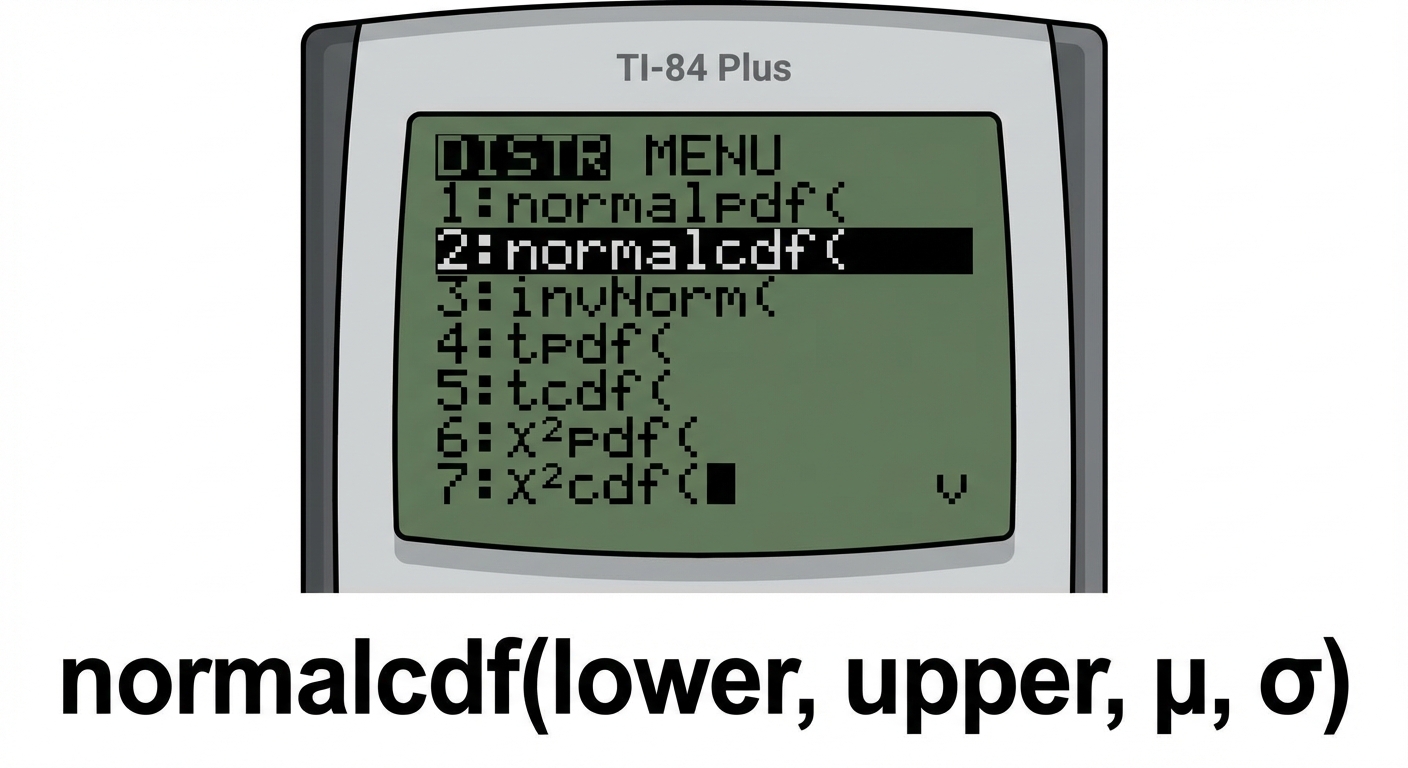
- Area: Using TI-84
normalcdf(lower: -1E99, upper: 0.75, mu: 0.80, sigma: 0.0381)ornormalcdf(lower: -10, upper: -1.31, mu: 0, sigma: 1). - Result: $P(\hat{p} < 0.75) \approx 0.0951$
Sampling Distribution for Differences in Proportions
When comparing two populations, we analyze the sampling distribution of the difference $\hat{p}1 - \hat{p}2$.
Formulas
- Center: $\mu{\hat{p}1 - \hat{p}2} = p1 - p_2$
- Spread:
- Note: Variances add, standard deviations do not. We sum the variances and take the square root.
Conditions
Must be checked for BOTH samples independently:
- Randomness: Independent random samples.
- 10% Condition: $n1 \le 0.10N1$ and $n2 \le 0.10N2$.
- Large Counts: $n1p1, n1(1-p1), n2p2, n2(1-p2)$ must all be $\ge 10$.
Sampling Distribution for Sample Means
We use the sample mean $\bar{x}$ to estimate the population mean $\mu$.
The Formulas
For an SRS of size $n$ from a population with mean $\mu$ and standard deviation $\sigma$:
- Center (Mean): $\mu_{\bar{x}} = \mu$
- Spread (Standard Deviation):
Important Concept: Behavior of Means
- Averages are less variable than individual observations.
- As $n$ increases, $\sigma_{\bar{x}}$ decreases (the curve becomes narrower and taller).
- The mean of the sampling distribution remains unbiased regardless of sample size.
Conditions for Normality (Crucial Distinction)
How do we know if the sampling distribution of $\bar{x}$ is Normal? We check one of two cases:
Case 1: The Population is Normal
If the original population distribution is Normal, the sampling distribution of $\bar{x}$ is Normal for any sample size $n$.
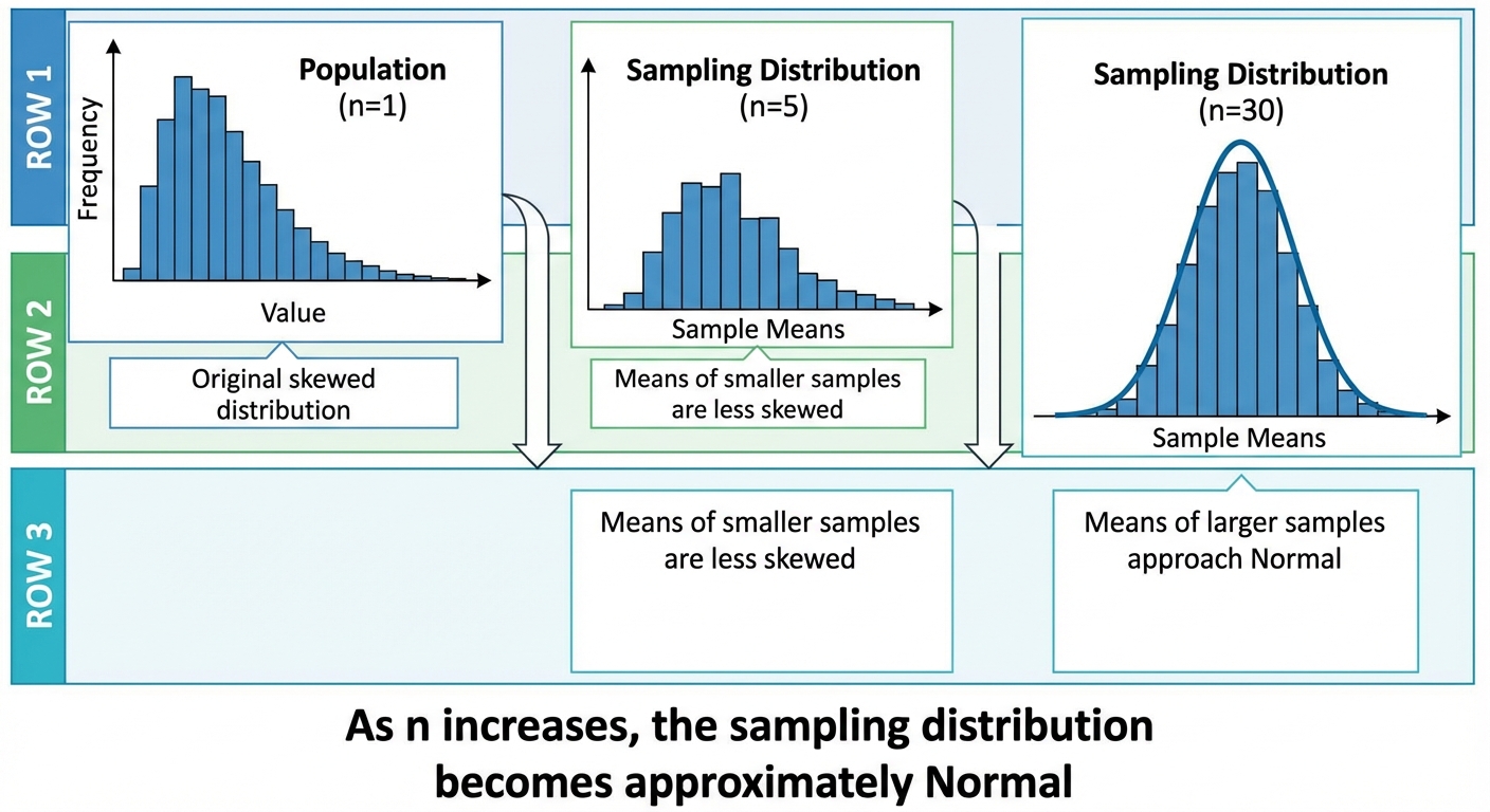
Case 2: The Central Limit Theorem (CLT)
If the population shape is unknown or skewed, the sampling distribution of $\bar{x}$ will be approximately Normal if the sample size is large ($n \ge 30$).
The Three Conditions
- Random: SRS.
- 10% Condition: $n \le 0.10N$ (Used to justify the formula $\sigma/\sqrt{n}$).
- Normal/Large Sample: Population is Normal OR $n \ge 30$ (CLT).
➥ Example 5.3: Naked Mole Rats
Life expectancy of mole rats: $\mu = 21$ years, $\sigma = 3$ years. Distribution is unknown. Sample size $n=40$.
- Check: $n=40 \ge 30$, so by the CLT, the sampling distribution is approx. Normal.
- Parameters: $\mu{\bar{x}} = 21$, $\sigma{\bar{x}} = \frac{3}{\sqrt{40}} \approx 0.474$.
- Problem: Probability that mean life expectancy is between 20 and 22 years.
normalcdf(lower: 20, upper: 22, mu: 21, sigma: 0.474) = 0.965.
Sampling Distribution for Differences in Means
When comparing two independent means, we analyze $\bar{x}1 - \bar{x}2$.
Formulas
- Center: $\mu{\bar{x}1 - \bar{x}2} = \mu1 - \mu_2$
- Spread:
Conditions
- Random: Independent random samples.
- 10% Condition: Checked for both populations.
- Normal/Large Sample: Both populations must be Normal OR both sample sizes ($n1, n2$) must be $\ge 30$.
➥ Example 5.4: Genetic Mutations
- Group 1 (40yo): $\mu1 = 65, \sigma1 = 15, n_1 = 35$.
- Group 2 (20yo): $\mu2 = 25, \sigma2 = 5, n_2 = 40$.
- Task: Probability that the difference in means (Group 1 - Group 2) is between 35 and 45.
Solution:
- Mean Diff: $65 - 25 = 40$
- SD Diff: $\sqrt{\frac{15^2}{35} + \frac{5^2}{40}} = \sqrt{6.428 + 0.625} \approx 2.656$
- Calculation:
normalcdf(35, 45, 40, 2.656) = 0.940. - Check: Both $n$ are $\ge 30$, so Normal approximation is valid via CLT.
Calculator Reference (TI-84)
1. Finding Probability (Area)
Use when you have the cut-off value ($x$, $\bar{x}$, or $\hat{p}$) and want the probability (percentage).
- Command:
2nd$\to$VARS$\to$2:normalcdf - Inputs:
(lower_bound, upper_bound, mean, SD) - Note: Use $-1E99$ for negative infinity and $1E99$ for positive infinity.
2. Finding Cut-off Values (Percentiles)
Use when you have the probability/area (e.g., "top 10%", "90th percentile") and want the cut-off value.
- Command:
2nd$\to$VARS$\to$3:invNorm - Inputs:
(area_to_the_left, mean, SD)
Common Mistakes & Pitfalls
Confusing the Law of Large Numbers (LLN) with the Central Limit Theorem (CLT)
- Mistake: Saying "The sample is large, so by the Law of Large Numbers it's normal."
- Correction: LLN says $\bar{x}$ approaches $\mu$ as $n$ grows. CLT says the shape of the distribution becomes Normal as $n$ grows.
Misapplying the Large Counts Condition
- Mistake: Using $n \ge 30$ to check normality for proportions.
- Correction: $n \ge 30$ is for means. For proportions, you MUST use $np \ge 10$ and $n(1-p) \ge 10$.
Forgetting to divide by $\sqrt{n}$
- Mistake: Using $\sigma$ instead of $\frac{\sigma}{\sqrt{n}}$ in
normalcdf. - Correction: If the problem asks about the probability of a sample mean, you must use the standard deviation of the sampling distribution (Standard Error), which is smaller than the population SD.
- Mistake: Using $\sigma$ instead of $\frac{\sigma}{\sqrt{n}}$ in
Notation Errors
- Mistake: Writing $\mu = 0.80$ for a proportion problem.
- Correction: Use $p$ for population proportion and $\mu$ for population mean. Use $\hat{p}$ for sample proportion and $\bar{x}$ for sample mean.
Standard Deviation vs. Standard Error
- If you know the population $\sigma$, use it. If you are approximating $\sigma$ with sample data ($s$), the standard deviation of the sampling distribution is technically called the Standard Error (Unit 6 concept, but good to know).