Unit 2: Linear Regression Models and Analysis
Least-Squares Regression Lines (LSRL)
The goal of linear regression is to model the relationship between two quantitative variables so that we can use the explanatory variable ($x$) to predict the response variable ($y$). While many lines could be drawn through a scatterplot, statisticians use a specific criterion to find the "best" fit.
The Definition of the LSRL
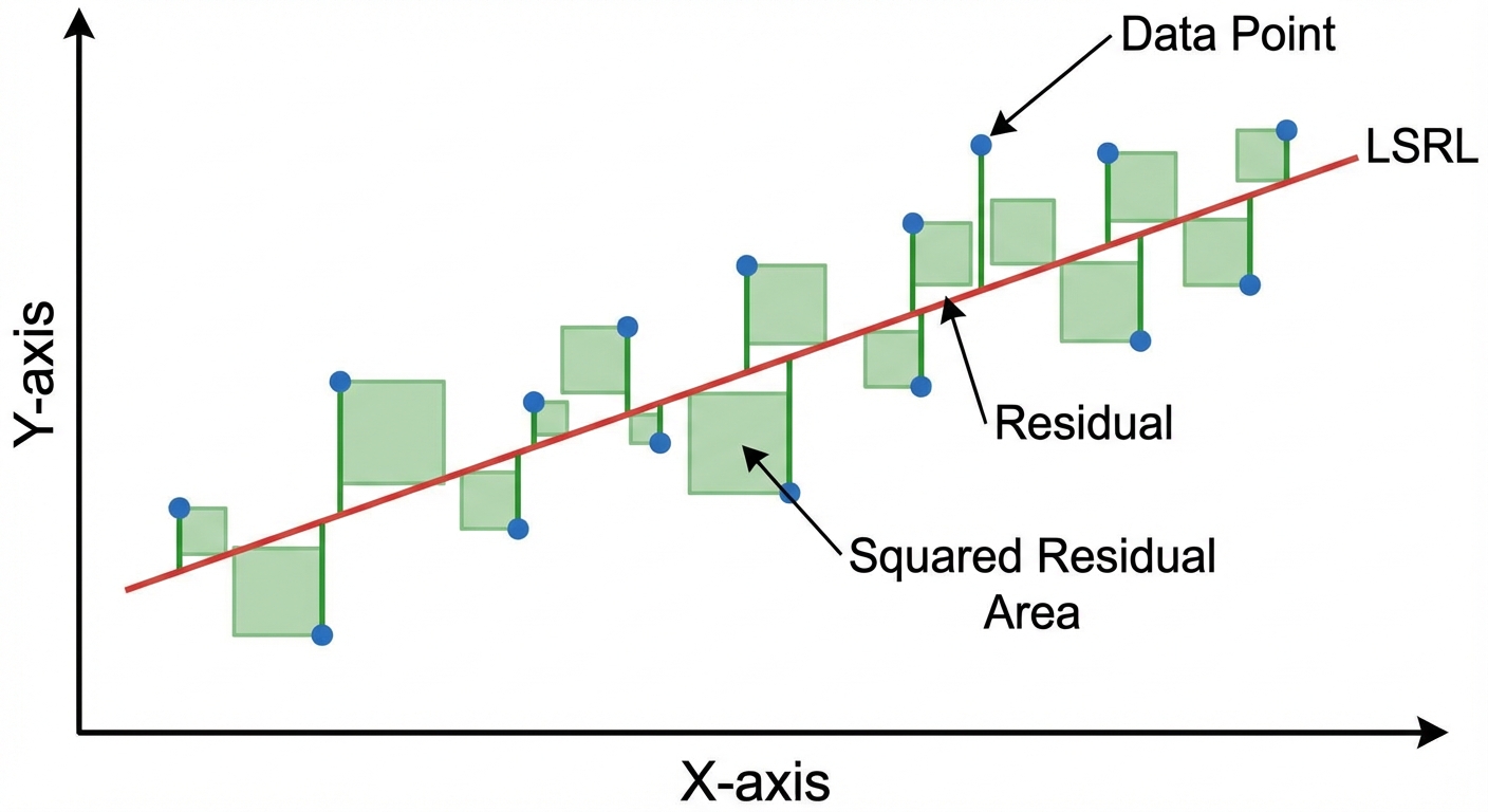
A Least-Squares Regression Line (LSRL) is the unique line such that the sum of the squared vertical distances (residuals) between the data points and the line is minimized.
Imagine drawing squares between every data point and the line. The LSRL represents the position where the total area of those squares is smallest.
Equation and Notation
On the AP Statistics formula sheet, the regression line is written as:
Where:
- $\hat{y}$ (read "y-hat") is the predicted value of the response variable.
- $b_0$ is the y-intercept.
- $b_1$ is the slope.
- $x$ is the value of the explanatory variable.
Note: You may also see the equation written as $\hat{y} = a + bx$. The coefficient attached to $x$ is always the slope, regardless of the letter used.
Calculating Slope and Y-Intercept
While calculators usually handle the heavy lifting, you must understand how the line relates to the summary statistics of the data:
1. The Slope ($b1$):
- The slope depends on the correlation ($r$) and the ratio of the standard deviations of $y$ ($sy$) and $x$ ($sx$).
- Because standard deviations are always positive, the slope ($b_1$) and correlation ($r$) always share the same sign (+ or -).
2. The Y-Intercept ($b0$):
- The LSRL always passes through the point $(\bar{x}, \bar{y})$.
Interpreting the Model
On Free Response Questions (FRQs), you are frequently asked to interpret the slope and intercept in context. Use these templates:
- Interpreting Slope: "For every 1 unit increase in [explanatory variable name], the predicted [response variable name] increases/decreases by approximately [value of slope]."
- Interpreting Y-Intercept: "When the [explanatory variable name] is 0, the predicted [response variable name] is [value of y-intercept]." (Note: Only interpret this if $x=0$ makes sense in the context of the problem).
Prediction and Extrapolation
To make a prediction, substitute a value of $x$ into the equation to find $\hat{y}$.
Extrapolation occurs when we use a regression model to make a prediction for an $x$-value typically outside the domain of the data used to build the model. This is dangerous because we cannot assume the linear pattern continues indefinitely.
Residuals, Residual Plots, and Assessing Linearity
A model is useful only if it fits the data well. We analyze residuals to assess the appropriateness of a linear model.
Understanding Residuals
A residual is the difference between the actual observed value ($y$) and the value predicted by the regression line ($\hat{y}$).
Formula:
- Memory Aid: Think "AP" $\rightarrow$ Actual minus Predicted.
- Positive Residual: The actual point is above the line (the model under-predicted).
- Negative Residual: The actual point is below the line (the model over-predicted).
- The sum of residuals for an LSRL is always 0.
The Residual Plot
A residual plot is a scatterplot that typically graphs the explanatory variable ($x$) on the horizontal axis against the residuals on the vertical axis.
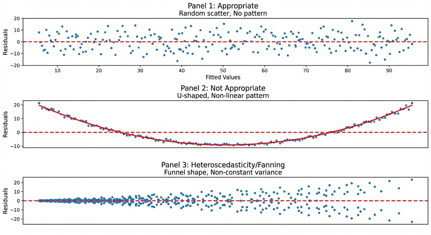
How to Read a Residual Plot:
- Random Scatter: If the plot shows no obvious pattern (just a cloud of dots centered around 0), the linear model is appropriate.
- Curved Pattern (U-shape or inverted U): If the residuals show a clear curve, the original data is non-linear. A linear model is not appropriate.
- Fanning (Cone Shape): If the residuals are small on one side and get larger on the other, the predictions are becoming less accurate. This is helpful to note, though the linear model might still be technically "appropriate" for the average, it is less reliable for predictions at the wide end of the fan.
Standard Deviation of the Residuals ($s$)
The value $s$ measures the "typical" distance between the actual data points and the regression line.
- Interpretation Template: "The actual [response variable] is typically about [value of $s$] away from the value predicted by the LSRL."
The Coefficient of Determination ($r^2$)
The value $r^2$ gives the proportion of variation in $y$ that can be explained by the variation in $x$.
- Interpretation Template: "About [value of $r^2$ as a %] of the variation in [response variable] is accounted for by the linear relationship with [explanatory variable]."
- Relationship to $r$: $\sqrt{r^2} = |r|$. You must look at the slope of the line to determine if $r$ is positive or negative.
Departures from Linearity and Influential Points
Sometimes, single data points can drastically affect our analysis. We classify these unusual points into three categories: outliers, high-leverage points, and influential points.
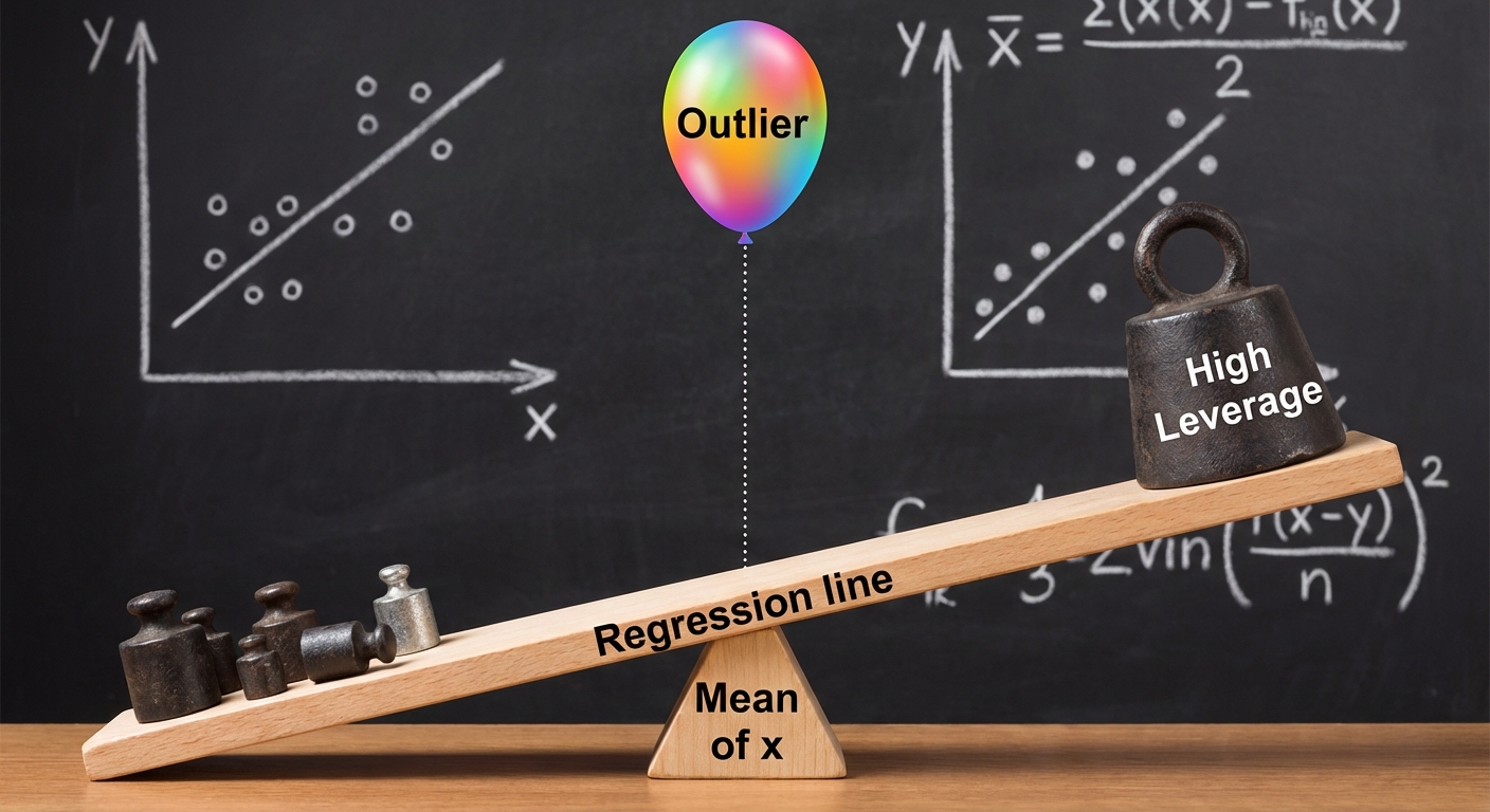
1. High-Leverage Points
A point has high leverage if its $x$-value is far from the mean of the x-values ($\bar{x}$). These points are usually separated horizontally from the rest of the data. High-leverage points have the potential to change the regression line dramatically because they act like weight at the end of a seesaw.
2. Outliers (in Regression)
An outlier in regression is a point with a large residual. It falls far above or below the regression line, fitting the pattern of the data poorly.
3. Influential Points
A point is considered influential if removing it from the dataset substantially changes the slope, y-intercept, or correlation.
- High-leverage points are often influential. If a point is far out in the x-direction and does not fall in line with the trend of the other points, it will pull the regression line toward itself, changing the slope significantly.
- Outliers (vertical deviations) generally weaken the correlation ($r$) and increase the standard deviation of residuals ($s$), but they may not change the slope much if they are near the center of the x-values ($\bar{x}$).
Reading Computer Output
On the AP exam, you are rarely asked to calculate a regression line by hand from a raw data table. Instead, you will be given output from statistical software (like Minitab or JMP) and asked to extract the equation.
A typical table looks like this:
| Predictor (or Term) | Coef | SE Coef | T | P |
|---|---|---|---|---|
| Constant | 24.5 | 1.22 | 8.1 | 0.000 |
| Hours Studied | 5.3 | 0.85 | 3.2 | 0.003 |
- S = 3.12
- R-Sq = 89.4%
How to extract the variables:
- Y-Intercept ($b0$): Look for the numbers next to "Constant" (or "Intercept"). In this example, $b0 = 24.5$.
- Slope ($b1$): Look for the number next to the variable name (e.g., "Hours Studied"). In this example, $b1 = 5.3$.
- Equation: $\widehat{Score} = 24.5 + 5.3(Hours Studied)$.
- $s$ and $r^2$: Usually listed at the bottom. ignore "R-Sq(adj)".
Common Mistakes & Pitfalls
- Forgetting the "Hat": When writing the equation, you MUST write $\hat{y}$ or $\widehat{context}$. Writing $y = a + bx$ implies the line hits every point perfectly, which is false. No hat = no credit.
- Confusing x and y: Remember that regression lines are one-way streets. You cannot solve the equation for $x$ to predict $x$ based on $y$. Mathematically you can, but statistically, it produces the wrong line of best fit.
- Misinterpreting $r^2$: Do not say "64% of the data points are on the line." Say "64% of the variation in the response variable is explained by the model."
- Correlation $\neq$ Causation: Even with a perfect $r^2$ of 100%, regression only demonstrates an association, not a cause-and-effect link. Only a well-designed experiment can prove causation.
- Extrapolation: Students often plug in any $x$-value given in a problem. Always check if the $x$-value is within the range of the original data. If not, state that the prediction may be unreliable.