Mastering Confidence Intervals for Population Proportions
Introduction to Confidence Intervals
In statistics, we often want to estimate a population parameter (like the true proportion of voters who support a candidate), but we only have access to a sample statistic. A single number—called a Point Estimate—is rarely exactly equal to the true parameter due to sampling variability.
To account for this uncertainty, we build a Confidence Interval. Think of this like fishing: a point estimate is like using a spear (trying to hit the exact spot), while a confidence interval is like using a net (casting a wider range to ensure you capture the fish).
The Anatomy of an Interval
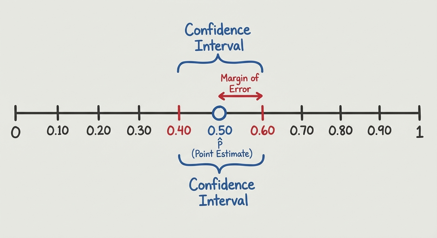
A confidence interval is constructed using the following general structure:
- Point Estimate (Statistic): Your best guess based on the sample data (observed variance) (e.g., $\hat{p}$).
- Margin of Error (ME): The product of the Critical Value and the Standard Error. It represents the maximum expected difference between the true population parameter and the sample estimate at a specific confidence level.
Constructing a Confidence Interval for a Population Proportion
When dealing with categorical data (success/failure), the specific method used is called the One-Sample $z$-Interval for a Proportion.
1. Identify the Parameter
Define the parameter $p$ in the context of the problem.
- Ex: Let $p$ = the true proportion of all US adults who own a smartphone.
2. Verify Conditions
Before calculating, you must verify three conditions to ensure the inference is valid.
- Random: The data must come from a random sample or a randomized experiment. This prevents bias.
- Independence (10% Condition): If sampling without replacement, the population size ($N$) must be at least 10 times the sample size ($n$).
- Normality (Large Counts Condition): The sampling distribution of $\hat{p}$ must be approximately normal. We check this by ensuring we expect at least 10 successes and 10 failures.
3. The Formula
The specific formula for a one-sample $z$-interval is:
- $\hat{p}$: The sample proportion (number of successes / sample size).
- $n$: Sample size.
- $z^*$: The Critical Value (z-score) corresponding to the confidence level.
- $\sqrt{\frac{\hat{p}(1-\hat{p})}{n}}$: The Standard Error (SE) of the sample proportion.
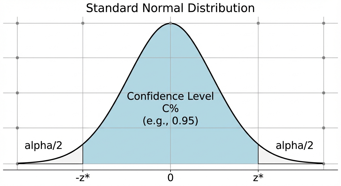
4. Critical Values ($z^*$)
The critical value ($z^*$) determines the width of the interval based on how confident you want to be. These values are derived from the Standard Normal Distribution.
| Confidence Level | Critical Value ($z^*$) |
|---|---|
| 90% | 1.645 |
| 95% | 1.960 |
| 99% | 2.576 |
Interpreting Confidence Intervals and Determining Sample Size
Success in AP Statistics relies heavily on the precise wording of your conclusions.
Interpreting the Interval
When asked to "interpret the confidence interval," use this template:
"We are [C%] confident that the interval from [lower bound] to [upper bound] captures the true proportion of [context of the problem]."
Example: "We are 95% confident that the interval from 0.45 to 0.55 captures the true proportion of students who drive to school."
Interpreting the Confidence Level
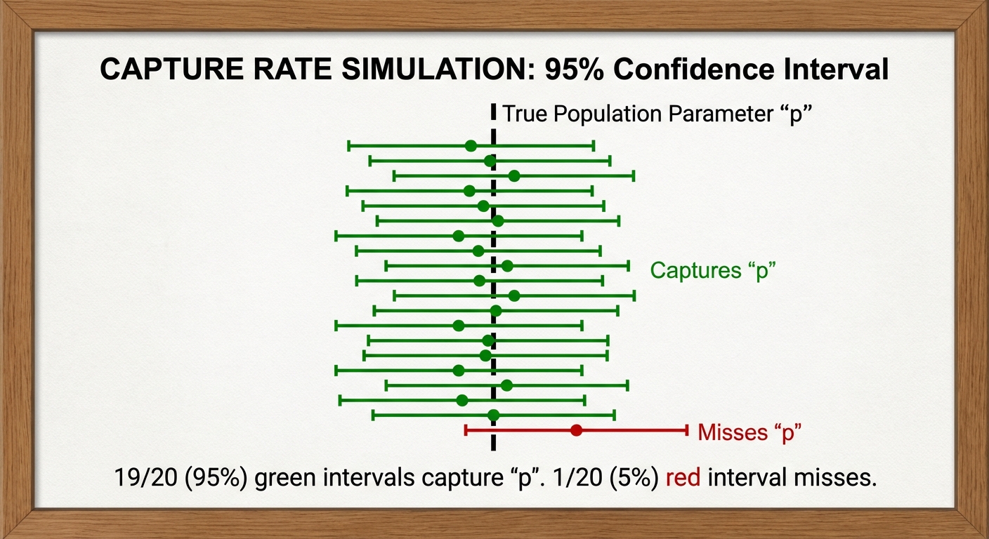
Sometimes a question asks what "95% confidence" means. This refers to the method, not the specific interval calculated.
"If we were to take many, many random samples of the same size from this population and construct a confidence interval for each, approximately 95% of those intervals would capture the true population proportion."
Determining Sample Size for a Desired Margin of Error
Researchers often plan a study by deciding the Margin of Error (ME) they are willing to accept first, then calculating the required sample size ($n$).
The formula for the Margin of Error is:
To find $n$, use algebra to rearrange the formula:
Key Rules for calculating $n$:
- Guessing $\hat{p}$: If previous data exists, use that estimate for $\hat{p}$. If no estimate is given, use $\hat{p} = 0.5$. This is the "conservative" estimate because $0.5(1-0.5) = 0.25$ yields the largest possible product, ensuring the sample size is large enough for any proportion.
- Rounding: Always round up to the next whole number. Even if you get $302.1$, you need 303 people.
Common Mistakes & Pitfalls
- Misinterpreting Probability:
- Wrong: "There is a 95% probability that the true parameter is between 0.4 and 0.6."
- Why: The true parameter is a fixed number (not a random variable). It is either in the interval or it isn't. Probability describes the method, not the specific result.
- Using Standard Deviation instead of Standard Error:
- When constructing an interval, we do not know $p$, so we use $\hat{p}$ inside the square root. This makes it Standard Error, not Standard Deviation.
- Using $t$-intervals for Proportions:
- Proportions always use $z$-statistics. $t$-statistics are only for Means.
- Checking Conditions with $p$ instead of $\hat{p}$:
- In intervals, we don't know $p$. You must use $\hat{p}$ (the sample proportion) to check the Large Counts condition ($n\hat{p} \geq 10$).