Unit 1 Review: Advanced Distribution Analysis
Comparing Distributions of Quantitative Data
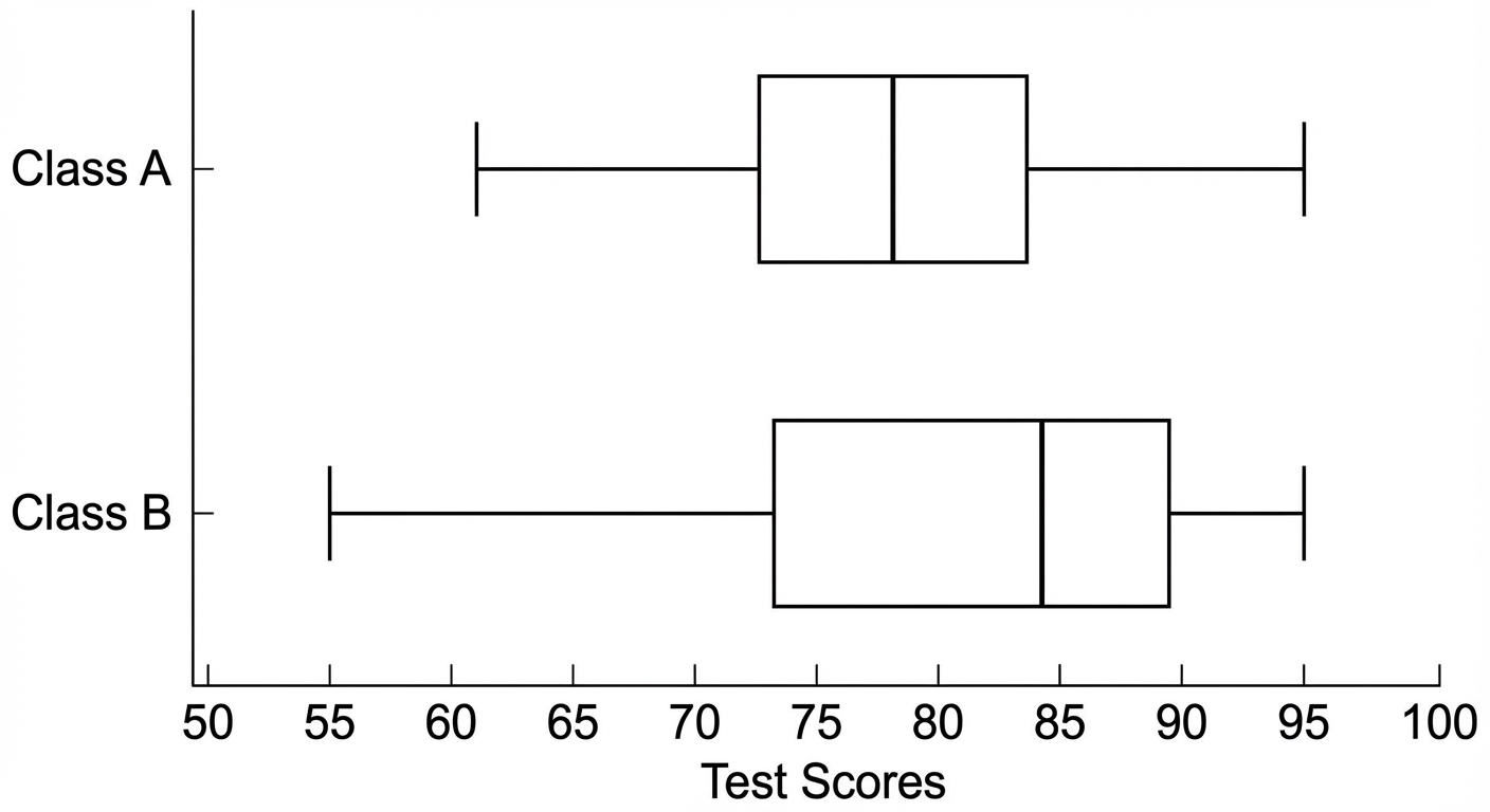
One of the most frequent tasks on the free-response section of the AP Statistics exam is comparing two or more distributions based on graphs (such as parallel boxplots, back-to-back stemplots, or side-by-side histograms). To earn full credit, you must go beyond simply listing statistics; you must explicitly compare them using linking words.
The Comparison Framework: SOCS (or CUSS)
When describing or comparing distributions, always address four key characteristics. A helpful mnemonic is SOCS:
- Shape: Is the distribution symmetric, skewed right, skewed left, or uniform? Is it unimodal or bimodal?
- Outliers (or Unusual Features): Are there any specific outliers (calculated via the $1.5 \times IQR$ rule) or gaps in the data?
- Center: Which measure of center is appropriate (mean or median)?
- Spread: How variable is the data? Use standard deviation or Interquartile Range (IQR).
Rules for Comparison
To compare distributions effectively, you must follow these three golden rules:
- Use Comparative Language: Do not just say "Group A has a median of 50 and Group B has a median of 60." You must say, "The median of Group B (60) is greater than the median of Group A (50)."
- Include Context: Always reference the variable name and the units (e.g., "test scores in points," "height in inches") rather than just saying "the data."
- Address All Four Aspects: Mention Shape, Outliers, Center, and Spread for the correct data visualization.
Choosing the Right Statistics
The shape of the distribution dictates which measures of center and spread you should compare.
| Distribution Shape | Measure of Center | Measure of Spread |
|---|---|---|
| Symmetric | Mean ($\bar{x}$) | Standard Deviation ($s_x$) |
| Skewed or with Outliers | Median | IQR (Interquartile Range) |
Note: The Median and IQR are resistant measures, meaning they are not heavily influenced by extreme values or skewness. The Mean and Standard Deviation are non-resistant.
The Normal Distribution and the Empirical Rule
The Normal Distribution is a continuous probability distribution that describes many natural phenomena. It forms the backbone of inference later in the course.
Properties of the Normal Model
A Normal density curve is determined fully by two parameters: the mean ($\mu$) and the standard deviation ($\sigma$).
- Shape: Symmetric, single-peaked (unimodal), and bell-shaped.
- Center: The mean, median, and mode are all located at the center of the curve.
- Notation: We denote a Normal distribution as $N(\mu, \sigma)$.
The Empirical Rule (68-95-99.7 Rule)
For any Normal distribution, the area under the curve (which represents proportion or probability) follows a specific pattern based on standard deviations from the mean.
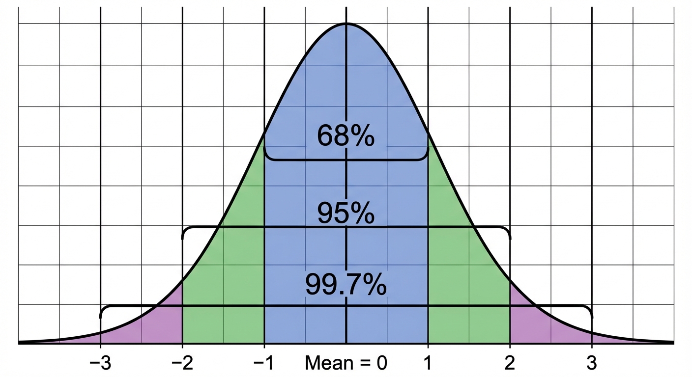
- Approximately 68% of observations fall within $\pm 1\sigma$ of the mean.
- Approximately 95% of observations fall within $\pm 2\sigma$ of the mean.
- Approximately 99.7% of observations fall within $\pm 3\sigma$ of the mean.
Worked Example: Using the Empirical Rule
Scenario: The distribution of heights of adult men is approximately Normal with mean $\mu = 70$ inches and standard deviation $\sigma = 2.5$ inches.
Question: Between what two heights do the middle 95% of men fall?
Solution:
- Identify the requirement: The middle 95% corresponds to $\pm 2$ standard deviations.
- Calculate bounds:
- Lower: $\mu - 2\sigma = 70 - 2(2.5) = 70 - 5 = 65$
- Upper: $\mu + 2\sigma = 70 + 2(2.5) = 70 + 5 = 75$
- Answer: The middle 95% of men are between 65 and 75 inches tall.
z-Scores and Percentiles
Not all observations fall nicely on the integer standard deviation lines ($1\sigma, 2\sigma$). To compare observations from different Normal distributions, or to find the location of any specific value, we use standardized scores (z-scores).
Definition of a z-Score
A z-score tells us how many standard deviations a particular data value ($x$) is from the mean ($\mu$).
Formula:
- Positive z-score: The value is above the mean.
- Negative z-score: The value is below the mean.
- z = 0: The value is the mean.
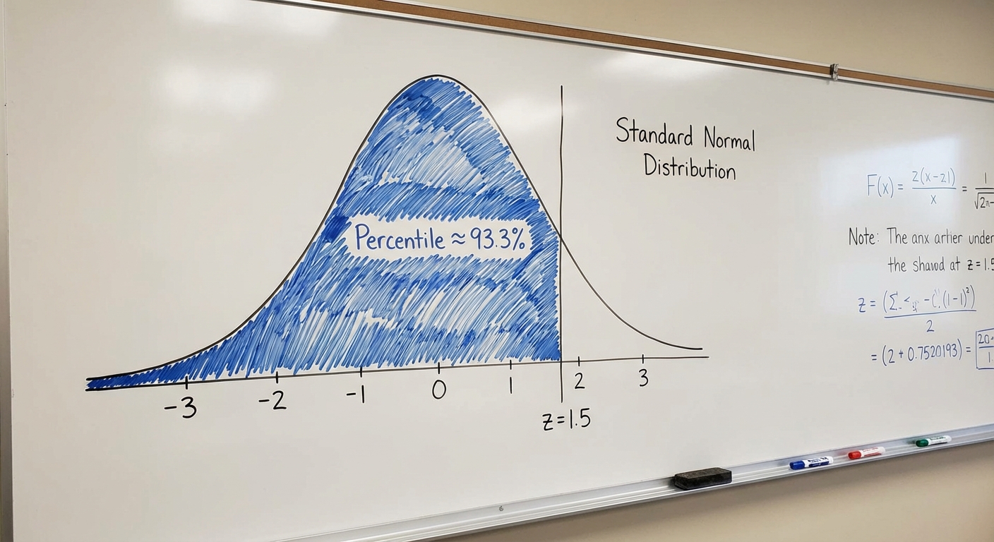
The Standard Normal Distribution
The Standard Normal Distribution is a special case where the mean is 0 and the standard deviation is 1.
- Notation: $N(0, 1)$
- We can transform any Normal distribution into the Standard Normal distribution using the z-score formula.
Percentiles
A percentile describes the location of a value in a distribution. The $p$-th percentile is the value with $p$ percent of the observations less than or equal to it.
- Visualizing Percentiles: On a density curve, the percentile corresponds to the area to the left of the z-score.
Worked Example: Comparing Apples and Oranges (Literally)
Imagine you scored a 1350 on the SAT (Mean=1100, SD=200) and a 30 on the ACT (Mean=21, SD=5). Which score is relatively better?
Calculate z-score for SAT:
Calculate z-score for ACT:
Conclusion: Since $1.80 > 1.25$, the ACT score is relatively better because it is more standard deviations above the mean than the SAT score.
Common Mistakes & Pitfalls
- Missing Context in Comparisons: Never write generic statements like "The mean is higher." Always write, "The mean weight of the elephants is higher than the mean weight of the hippos."
- Confusing Skewness and Mean/Median Relationship:
- Skewed Right: Mean > Median (The tail drags the mean up).
- Skewed Left: Mean < Median (The tail drags the mean down).
- Using the Empirical Rule on Non-Normal Data: You cannot use the 68-95-99.7 rule if the distribution is not stated to be Normal or is clearly skewed.
- Misinterpreting z-scores as Percentages: A z-score of 2.0 does not mean 2%. It corresponds (approximately) to the 97.7th percentile (area to the left is 0.9772).
- Area vs. Value: Remember that table values (or calculator output
normalcdf) give you the area (probability), not the x-value. Conversely,invNormtakes an area and gives you a z-score or x-value.