AP Statistics: Inference for Quantitative Data (Means)
The Student’s t-Distribution
Why Not the Normal Distribution?
In previous units involving sample proportions, we used the Normal (z) distribution because we could assume the sampling distribution was normal. However, when working with quantitative data (means), we face a problem: to calculate the standardized score (z-score), we need the population standard deviation ().
In the real world, if we don't know the population mean (), we almost certainly do not know the population standard deviation (). Therefore, we must estimate using the sample standard deviation (). substituting for introduces extra variability, meaning our statistic no longer follows a perfect Normal distribution. Instead, it follows the Student’s t-distribution.
Characteristics of the t-Distribution
The t-distribution was published in 1908 by W.S. Gosset (under the pseudonym "Student").
- Shape: Like the Standard Normal, it is bell-shaped and symmetric centered at 0.
- Spread: It has "fatter" tails and a lower peak than the Standard Normal. This accounts for the extra uncertainty introduced by estimating with .
- Degrees of Freedom (df): There is a different t-distribution for every sample size. We distinguish them by degrees of freedom.
- For a one-sample t-statistic: .
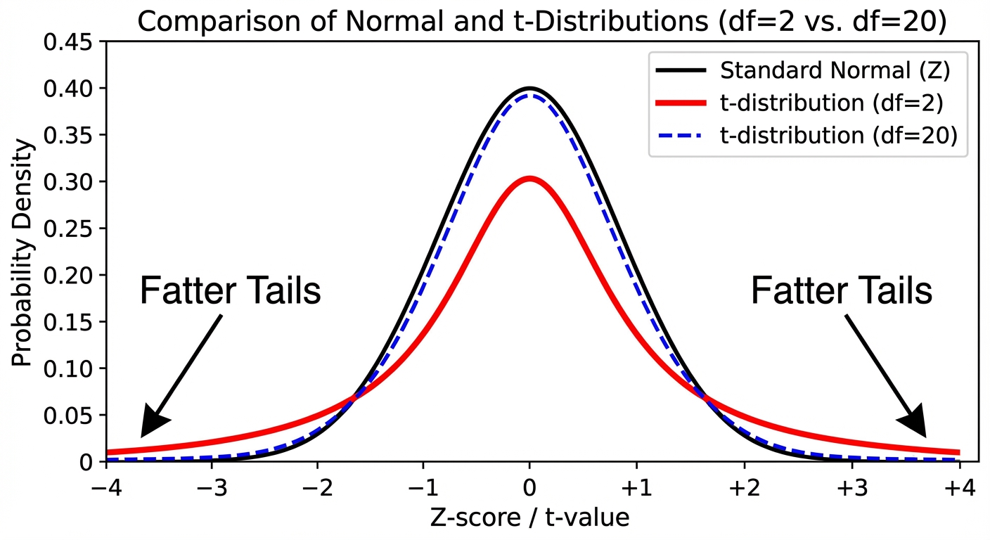
Key Trend: As the sample size () increases, the degrees of freedom increase, and the t-distribution approaches the Standard Normal distribution. The tails get thinner as our estimate becomes more reliable.
Inference for a Single Mean
1. Conditions for Inference
Before calculating a confidence interval or performing a test for a mean, you must verify three conditions. Use the mnemonic Rx3 (Random, 10%, Normal/Large).
- Random: The data must come from a random sample or a randomized experiment. This prevents bias.
- 10% Condition: If sampling without replacement, the sample size () must be less than 10% of the population size (). This allows us to treat observations as independent.
- Check: n < 0.10N
- Normal/Large Sample: We need the sampling distribution of to be approximately Normal.
- If population is Normal: The sample size doesn't matter.
- If population shape is unknown:
- : The Central Limit Theorem (CLT) guarantees the sampling distribution is approximately normal.
- : You must plot the sample data (dot plot or box plot). If there is no strong skewness and no outliers, the t-procedure is robust enough to use.
2. Standard Error of the Mean
When we estimate the standard deviation of the sampling distribution using , we call it the Standard Error (SE).
3. One-Sample t-Interval (Confidence Interval)
A confidence interval estimates the true population mean .
- depends on the confidence level (e.g., 95%) and the degrees of freedom ().
➥ Example 7.1: Gas Mileage
A random sample of 10 cars of a new model shows a mean gas mileage of 27.2 mpg with a standard deviation of 1.8 mpg. The population is approximately normally distributed. Construct a 95% confidence interval.
Solution: (PANIC Method)
- P (Parameter): Let be the true mean gas mileage of all cars of this new model.
- A (Assumptions):
- Random: Stated in problem.
- *10%: * Assume 10 cars < 10% of all cars.
- Normal: Population stated to be approximately normal.
- N (Name): One-Sample t-Interval.
- I (Interval):
- . For 95% confidence, inverse-t gives .
- Result: (25.91, 28.49)
- C (Conclusion): We are 95% confident that the interval from 25.91 to 28.49 mpg captures the true mean gas mileage of this new car model.
4. One-Sample t-Test (Significance Test)
Used to test a claim about a population mean.
- Null Hypothesis:
- Test Statistic:
➥ Example 7.2: AC Usage
A manufacturer claims their unit uses 6.5 kW/day. A consumer agency suspects it uses more. A random sample of 50 units has a mean of 7.0 kW and kW.
Solution: (PHANTOMS Method)
- P: = true mean electricity usage of the new AC units.
- H: vs. Ha: \mu > 6.5
- A: Random sample? Yes. 10% condition? Assume 50 < 10% of production. Normal/Large? , so CLT applies.
- N: One-Sample t-Test.
- T:
- O (Obtain P-value): Using , P(t > 2.525) \approx 0.0074.
- M (Make Decision): Since 0.0074 < 0.05(\alpha), we reject .
- S (State Conclusion): There is convincing evidence that the true mean electricity usage is greater than 6.5 kW.
Inference for Paired Data
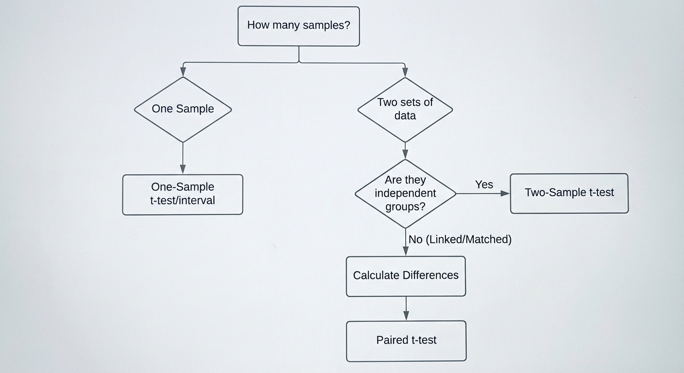
Distinguishing Paired Data from Two Sample Data
Crucial Concept: Do not confuse Paired Data with Two Independent Samples.
- Paired Data (Dependent): Data comes in couples. Example: Pre-test and Post-test scores for the same student; or twins; or right-arm vs left-arm. You are interested in the mean of the differences ().
- Two Independent Samples: The two groups have no relationship. Example: The mean height of men vs. the mean height of women.
The Paired t-Procedure
For paired data, we calculate the difference for each pair first (). Then, we perform a One-Sample t-test/interval on that single list of differences.
➥ Example 7.5: SAT Scores (Paired)
30 random students take an SAT prep class. We have their score Before and After. We want to know the mean improvement.
Common Mistake: Calculating the mean of the "Before" group and the mean of the "After" group and treating them as two samples. Wrong! These are the same students.
Correct Method:
- Calculate for every student.
- Find and (given).
- Procedure: Paired t-Interval (One-sample t-interval on differences).
- Calc:
- Result: (33.59, 50.91).
- Conclusion: We are 90% confident the true mean improvement is between 33.59 and 50.91 points.
Inference for the Difference of Two Means
When we have two independent groups, we compare their population means ().
1. Conditions
- Random: Two independent random samples OR randomized assignment in an experiment.
- 10%: Applies to both populations separately (if observational).
- Normal/Large: Both and , OR both populations are Normal, OR both sample graphs show no skew/outliers.
2. Formulas for Two Independent Samples
Standard Error:
Confidence Interval:
Two-Sample t-Statistic:
3. Degrees of Freedom (The Messy Part)
There are two ways to calculate df for two samples:
- Calculator Method (Satterthwaite approximation): A complex formula that usually yields a decimal. Use this for the most accurate results on the AP exam.
- Conservative Method: . This is easier for hand calculations but yields a wider (less powerful) interval.
Note: Do NOT Pool. In AP Statistics, we generally do not pool variances () unless there is a very specific theoretical reason. Assume unpooled for calculations.
➥ Example 7.4: Computer Downtime
- Company A: , , .
- Company B: , , .
- Tests claim: Company A has more downtime ().
Analysis:
- Ha: \muA - \mu_B > 0
- Using a calculator (2-SampTTest), we get and .
- Conclusion: Since 0.14 > 0.05, we fail to reject . We do not have convincing evidence that Company A's downtime is higher.
Connecting Confidence Intervals and Test Conclusions
Confidence Intervals (CI) and Significance Tests are mathematically consistent.
- Two-Sided Test (): If the Null value lies outside the corresponding Confidence Interval, you generally Reject .
- One-Sided Test: The connection is looser, but the logic holds. If the CI is entirely above the Null value, it supports a "GREATER THAN" hypothesis.
➥ Example 7.8: Consistency Check
Suppose we test vs at .
- If the 95% Confidence Interval is (-3.4, 23.4):
- Since 0 is inside the interval, it is a plausible value.
- We would Fail to Reject .
- If the 95% Confidence Interval is (0.5, 19.5):
- Since 0 is NOT in the interval, 0 is not plausible.
- We would Reject .
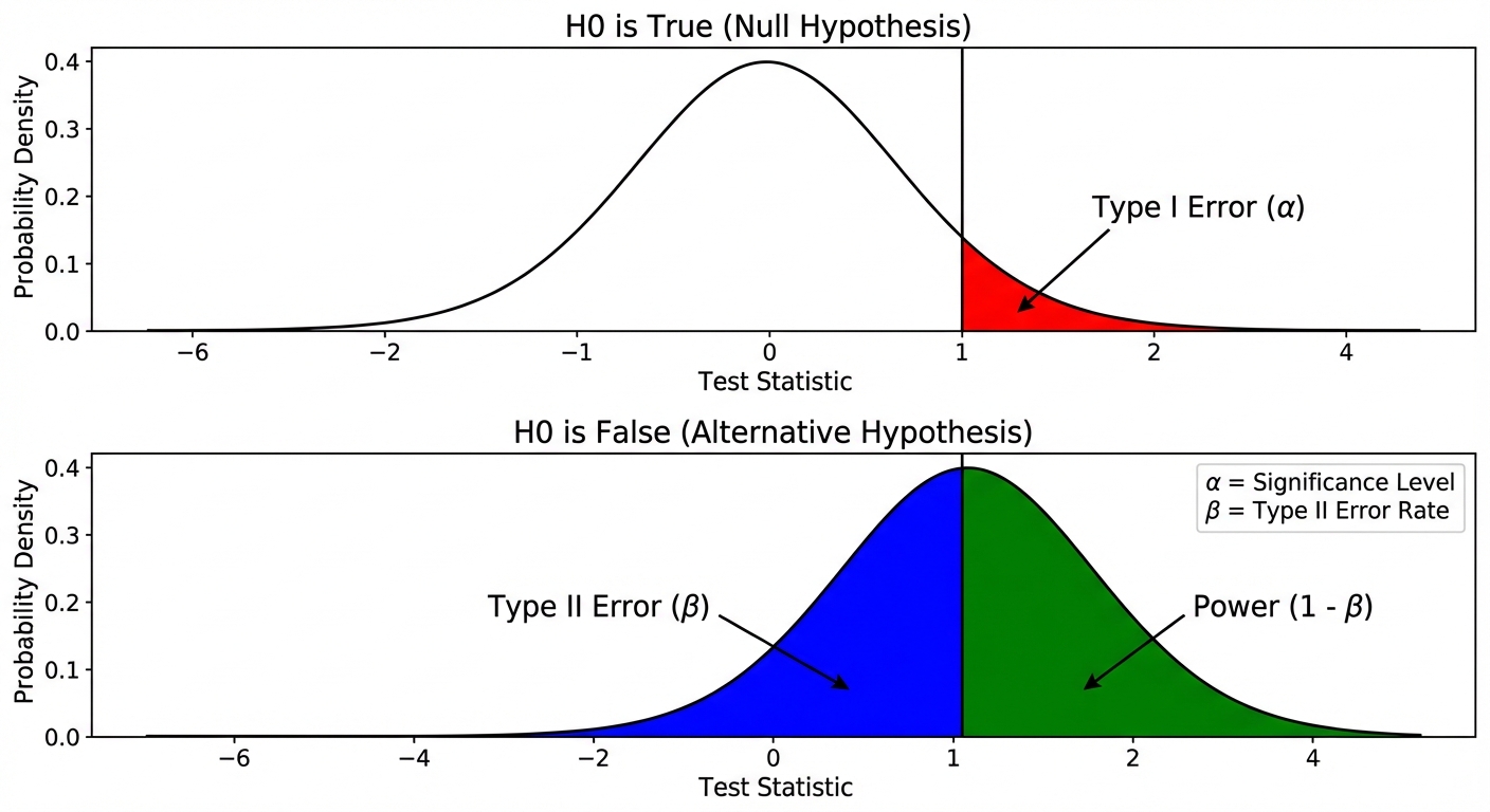
Power, Type I, and Type II Errors
Though introduced earlier, these concepts apply to Means frequently in Free Response Questions.
- Type I Error (): Rejecting when is actually True. (False Positive).
- Type II Error (): Failing to reject when is False. (False Negative).
- Power (): The probability of correctly rejecting a false null hypothesis.
Key Relationships:
- Increase (Sample Size): Power increases. (It's easier to detect a difference with more data).
- Increase (Significance Level): Power increases, but Type I error risk increases.
- Effect Size: If the true mean is very far from the null mean, Power increases.
Simulation and P-Values
Sometimes, instead of a formula, we use simulation to estimate a P-value.
Logic:
- Assume is true.
- Simulate the sampling process 100 or 1000 times.
- See how often a result as extreme as your observed sample occurs.
- Estimated P-value = (Count of extreme simulations) / (Total simulations).
➥ Example 7.6 Review (MAD)
If a simulation of 100 trials shows that a MAD value of 0.06 or greater occurred only 3 times, the P-value is approx 0.03. Since 0.03 < 0.05, the result is statistically significant.
Common Mistakes & Pitfalls
Confusing Paired vs. Two-Sample:
- Tip: Look for the data source. Are there two separate groups of people (2-Sample)? Or is it one person measured twice (Paired)?
- Error: Using 2-Sample t-test on paired data reduces the Power significantly.
Using z instead of t:
- Rule: If you use (sample SD) to estimate , you MUST use t.
- Correction: Only use z if the problem explicitly says "Population Standard Deviation is known" (rare).
Interpreting the CI Incorrectly:
- Wrong: "There is a 95% probability sample mean is in the interval."
- Wrong: "95% of data is in the interval."
- Correct: "We are 95% confident that the interval captures the true population mean."
Misidentifying Degrees of Freedom:
- Remember for one sample. Don't use .
- For two samples, write down the calculator's df value.
Not Checking Conditions:
- In FRQs, you get credit for identifying the procedure, but you lose substantial points if you don't explicitly check Random, 10%, and Normal conditions in context.