AP Statistics Unit 8: Inference for Categorical Data
Introduction to Chi-Square Distributions
Unlike $t$-tests and $z$-tests which are used for means and proportions involving quantitative data or binary categorical data, the Chi-Square ($\chi^2$) procedures are designed for non-binary categorical data involving counts.
The Chi-Square Statistic
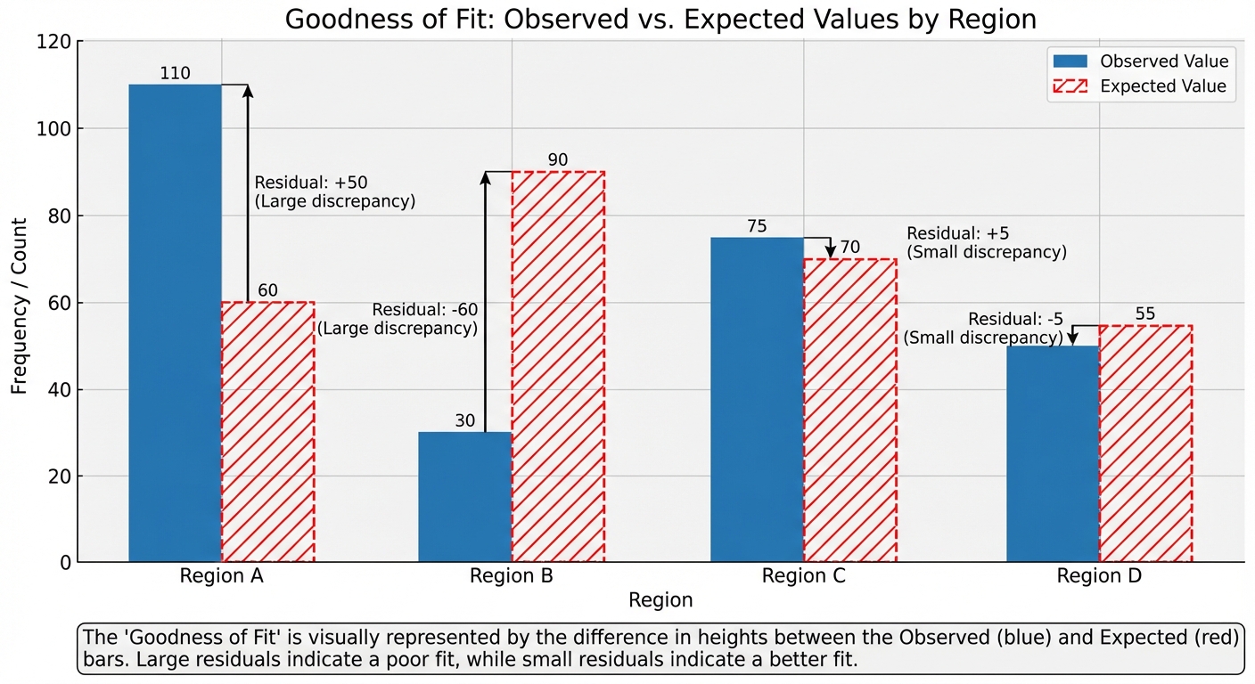
The Chi-Square statistic measures how far observed counts fall from the counts we would expect if the null hypothesis were true. It is essentially a sum of weighted discrepancies.
The formula for the statistic is:
- Observed ($O$): The actual count observed in the sample data.
- Expected ($E$): The count predicted by the null hypothesis.
- The difference $(O - E)$ is squared to handle negative differences.
- It is divided by $E$ to standardize the difference relative to the size of the category (a difference of 5 is huge if we expect 10, but negligible if we expect 10,000).
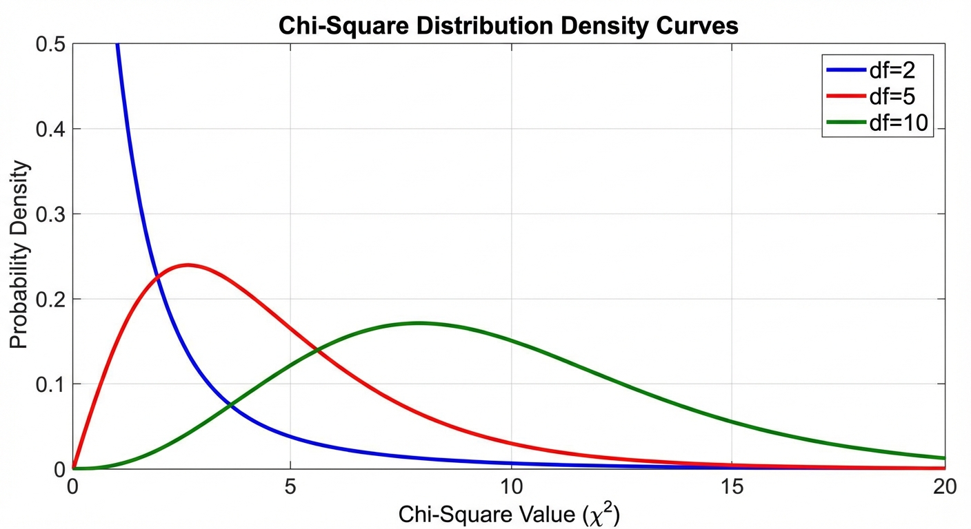
Properties of the $\chi^2$ Distribution
The Chi-Square statistic follows a specific density curve known as the Chi-Square Distribution. Its properties differ significantly from the Normal distribution:
- Non-Negative: $\chi^2$ values are always $\ge 0$ (because squares cannot be negative).
- Skewed Right: The curve is not symmetric; it has a long tail to the right.
- Defined by Degrees of Freedom ($df$): There is a family of curves determined by specific degrees of freedom.
- As $df$ increases, the curve flattens out, the peak moves to the right, and it becomes more symmetric (approaching Normality).
The Chi-Square Test for Goodness-of-Fit
This test is used when you have one sample and one categorical variable and you want to verify if the sample distribution differs significantly from a specific proposed population distribution.
Hypotheses
- Null Hypothesis ($H_0$): The categorical variable has the specified distribution (e.g., "The colors of M&Ms are distributed as 20% Red, 10% Blue, etc.").
- Alternative Hypothesis ($H_a$): The categorical variable does not have the specified distribution (at least one proportion is different).
Conditions for Inference
To effectively use the $\chi^2$ Goodness-of-Fit test, three conditions must be met:
- Random: The data comes from a random sample or randomized experiment.
- 10% Condition: If sampling without replacement, $n < 0.10N$ (sample size is less than 10% of the population).
- Large Counts: All expected counts must be at least 5.
- Note: It is okay if observed counts are less than 5, but expected must be $\ge 5$.
Mechanics and Calculation
1. Calculating Expected Counts:
Where $n$ is the total sample size and $p_i$ is the hypothesized proportion for that category.
2. Degrees of Freedom:
3. Calculating P-value:
The P-value is the probability of obtaining a $\chi^2$ statistic as or more extreme than the one calculated, assuming $H_0$ is true. Since the curve is right-tailed, we look at the area to the right of our statistic.
➥ Example: Liquor Store Distribution
A city planner believes liquor stores are distributed unevenly across four regions based on the region's size. The theoretical distribution based on area is:
- Upper Class: 12%
- Middle Class: 38%
- Lower Class: 32%
- Mixed Class: 18%
A random sample of 55 stores reveals observed counts of: 4, 16, 26, and 9 respectively. Is there evidence the stores do not follow the area distribution?
Step 1: Hypotheses
- $H0$: The distribution of liquor stores matches the distribution of region area ($p1=0.12, p_2=0.38…$).
- $H_a$: The distribution of liquor stores does not match the distribution of region area.
Step 2: Check Conditions
- Random: Stated as a random sample.
- 10%: 55 is reasonably less than 10% of all stores in a large city.
- Large Counts: We must calculate expected values first.
- Upper: $0.12 \times 55 = 6.6$
- Middle: $0.38 \times 55 = 20.9$
- Lower: $0.32 \times 55 = 17.6$
- Mixed: $0.18 \times 55 = 9.9$
All Expected counts $> 5$. Conditions met.
Step 3: Calculate Statistic
Using a calculator ($\chi^2\text{cdf}$ or Goodness-of-Fit test), $P\text{-value} \approx 0.099$.
Step 4: Conclusion
Since $P = 0.099 > \alpha = 0.05$, we fail to reject $H_0$. We do not have convincing evidence that the distribution of liquor stores differs from the distribution of the land area.
Inference for Two-Way Tables
When we deal with two-way tables (contingency tables), we are examining the relationship between variables or populations. The calculation for the statistic is the same, but the expected counts and degrees of freedom change.
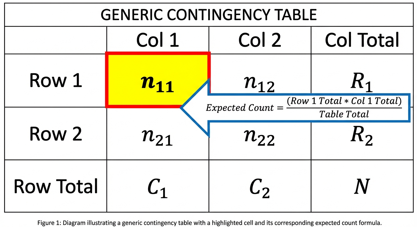
General Notation & Formulas
For a table with $r$ rows and $c$ columns:
Degrees of Freedom:
Expected Count for a specific cell:
The Chi-Square Test for Homogeneity
Purpose
Used to determine if a single categorical variable has the same distribution across multiple distinct populations (or multiple treatment groups).
Key Identifier: This test usually arises from a standard comparative experiment or when Stratified Random Sampling is used (sampling 100 people from each of 3 specific groups).
Hypotheses
- $H_0$: The true proportional distribution of [Variable] is the same for all [Groups/Populations].
- $H_a$: The true proportional distribution of [Variable] is different for at least two of the [Groups/Populations].
➥ Example: School Employees
We take independent random samples of four job types (Teachers, Admin, Custodians, Secretaries) and ask if they are satisfied.
- Data Setup: 4 separate sample groups. 1 variable (Satisfaction: Yes/No).
- $N = 260$ total surveyed.
- Job groups are the populations. Satisfaction is the variable.
Observed Data:
| Group | Satisfied | Not Satisfied | Total |
|---|---|---|---|
| Teachers | 82 | 18 | 100 |
| Admin | 38 | 22 | 60 |
| Custodians | 34 | 11 | 45 |
| Secretaries | 36 | 19 | 55 |
Calculated $\chi^2$: 8.707
df: $(4-1)(2-1) = 3$
P-value: 0.0335
Conclusion: Since $P < 0.05$, we reject $H_0$. There is sufficient evidence that the distribution of job satisfaction differs among the various school employee groups.
The Chi-Square Test for Independence
Purpose
Used to determine if there is an association between two categorical variables within a single population.
Key Identifier: This arises when a single random sample is taken from one population, and the individuals are classified according to two variables (cross-categorized).
Hypotheses
- $H_0$: There is no association between [Variable 1] and [Variable 2] (they are independent).
- $H_a$: There is an association between [Variable 1] and [Variable 2] (they are not independent).
➥ Example: Politics & Marijuana
A single random sample of 1,000 adults is taken. We ask them their Party (Dem/Rep/Ind) and their Support for Marijuana Legalization (Yes/No).
- Data Setup: One sample ($n=1000$). Two variables sorted into a $3 \times 2$ table.
- Hypotheses:
- $H_0$: Party affiliation and Support for legalization are independent.
- $H_a$: Party affiliation and Support for legalization are NOT independent.
Result: $\chi^2 = 94.5, P \approx 0.000$.
Conclusion: We reject $H_0$. There is strong evidence of an association between political party and support for legalization.
Comparing the Three Tests
Students often confuse the three types of Chi-Square tests. Use this table to distinguish them:
| Feature | Goodness-of-Fit | Homogeneity | Independence |
|---|---|---|---|
| Number of Samples | One sample | Multiple independent samples (or groups) | One sample |
| Number of Variables | One variable | One variable | Two variables |
| Question Asked | Do data match a theoretical model? | Are distributions the same across groups? | Are the two variables associated? |
| Degrees of Freedom | $Categories - 1$ | $(Row-1)(Col-1)$ | $(Row-1)(Col-1)$ |
| Hypothesis Keywords | "Fits distribution…" | "Same distribution…" | "Independent" or "Associated" |
Common Mistakes & Pitfalls
Using Proportions instead of Counts:
- Mistake: Using percentages or probabilities in the matrix or list L1/L2 calculation.
- Correction: Chi-Square always uses raw counts (integers). Never input "0.25" or "50%" into the formula.
Misinterpreting "Large Counts" Condition:
- Mistake: Checking if the Observed counts are $\ge 5$.
- Correction: The condition applies only to Expected counts. It is mathematically acceptable to observe a 0, as long as the model expected $\ge 5$.
Phrasing the Alternative Hypothesis:
- Mistake for Homogeneity: "$H_a$: All the groups are different."
- Correction: "$H_a$: The distribution is different for at least two of the groups." They don’t all have to be unique; just one deviation breaks the null.
Causation:
- Mistake: Assuming a significant Test for Independence proves one variable causes the other.
- Correction: Like correlation, association does not imply causation, especially in observational studies (surveys). It only indicates a link.
Direction of the Test:
- Mistake: Doing a two-tailed test.
- Correction: Chi-Square tests are essentially always right-tailed. A $\chi^2$ value close to 0 (left side) means the observed match expected perfectly (evidence for $H0$). Only large deviations (right tail) provide evidence against $H0$.