Comprehensive Guide to Chance Processes and Distributions
Randomness, Probability, and Simulation
The Concept of Probability
Probability is the mathematics of chance. It describes the long-term patterns of unpredictable events. While individual outcomes are uncertain, there is a regular pattern in the long run.
- Random Process: A situation in which we know what outcomes could happen, but we cannot predict which particular outcome will happen.
- Probability: The proportion of times the outcome would occur in a very long series of repetitions. It is always a number between 0 and 1.
The Law of Large Numbers (LLN)
The Law of Large Numbers states that as the number of trials increases, the observed relative frequency of an event approaches its true probability.
Two Key Conditions:
- The chance event does not change from trial to trial (independence).
- The conclusion is based on a large number of observations.
Misconception Alert: The "Law of Averages" is a myth. Short-run regularity does not exist. If you flip a coin and get 5 heads in a row, the 6th flip is not "due" to be tails. The probability remains 0.5.
➥ Example 4.1: Coin Flipping Strategy
Two games involve flipping a fair coin:
- Game A: Win if observing between 45% and 55% heads.
- Game B: Win if observing more than 60% heads.
- Decision: Would you choose 20 flips or 200 flips for each?
Solution:
- Game A: You want the result to be close to the true probability (50%). According to LLN, 200 flips is better because relative frequency stabilizes near the true probability with more trials.
- Game B: You want an outlier result (far from 50%). With fewer tosses, there is a greater chance of wide swings (variability). Thus, choose 20 flips.
Basic Probability Rules
Sample Spaces and Events
- Sample Space ($S$): The set of all possible outcomes.
- Event: A subset of outcomes in the sample space.
- Complement ($A^C$): The event that $A$ does not occur.
Mutually Exclusive vs. Independent Events
This is the most frequent conceptual confusion in Unit 4. Memorize the difference:
| Concept | Definition | Mathematical Check |
|---|---|---|
| Mutually Exclusive (Disjoint) | Two events cannot happen at the same time. There is no overlap. | |
| Independent | Knowing one event has occurred does not change the probability of the other occurring. | P(A |
General Probability Rules
General Addition Rule (For any two events):
P(A \cup B) = P(A) + P(B) - P(A \cap B)
Note: If events are mutually exclusive, $P(A \cap B) = 0$, so we just add.General Multiplication Rule (For intersection/joint probability):
P(A \cap B) = P(A) \cdot P(B|A)Conditional Probability:
The probability of $A$ given that $B$ has already occurred:
P(A|B) = \frac{P(A \cap B)}{P(B)}
➥ Example 4.2: Literacy Test Analysis
A test has 100 questions. Results from 1000 takers and their strategies are below:
| Strategy | Score 0-59 | Score 60-79 | Score 80-100 | Total |
|---|---|---|---|---|
| Guess | 80 | 115 | 70 | 265 |
| Answer C | 50 | 230 | 110 | 390 |
| Longest | 170 | 135 | 40 | 345 |
| Total | 300 | 480 | 220 | 1000 |
Detailed Solutions:
- P(Guess): $265/1000 = 0.265$
- P(Score 60-79): $480/1000 = 0.48$
- P(Not Score 60-79): $1 - 0.48 = 0.52$
- P(Answer C $\cap$ Score 80-100): Look for the intersection in the table. $110/1000 = 0.11$.
- P(Longest $\cup$ Score 0-59): Use Addition Rule.
P(Longest) + P(0\text{-}59) - P(Longest \cap 0\text{-}59)
= \frac{345}{1000} + \frac{300}{1000} - \frac{170}{1000} = \frac{475}{1000} = 0.475 - P(Guess | Score 0-59): Focus only on the "Score 0-59" column.
= \frac{\text{Intersection}}{\text{Condition Total}} = \frac{80}{300} \approx 0.267 - Independence Check: Are "Guess" and "Score 0-59" independent?
- Check: Does $P(Guess | 0\text{-}59) = P(Guess)$?
- $0.267 \neq 0.265$. They are not strictly independent (though close).
- Mutually Exclusive Check: can you "Answer C" and "Score 80-100" at the same time?
- Intersection is 110 (not 0). They are not mutually exclusive.
Multistage Probability (Tree Diagrams)
When events happen in sequence, Tree Diagrams are the most effective tool. Multiply along the branches to find intersections; add the resulting end-branches to find total probabilities.
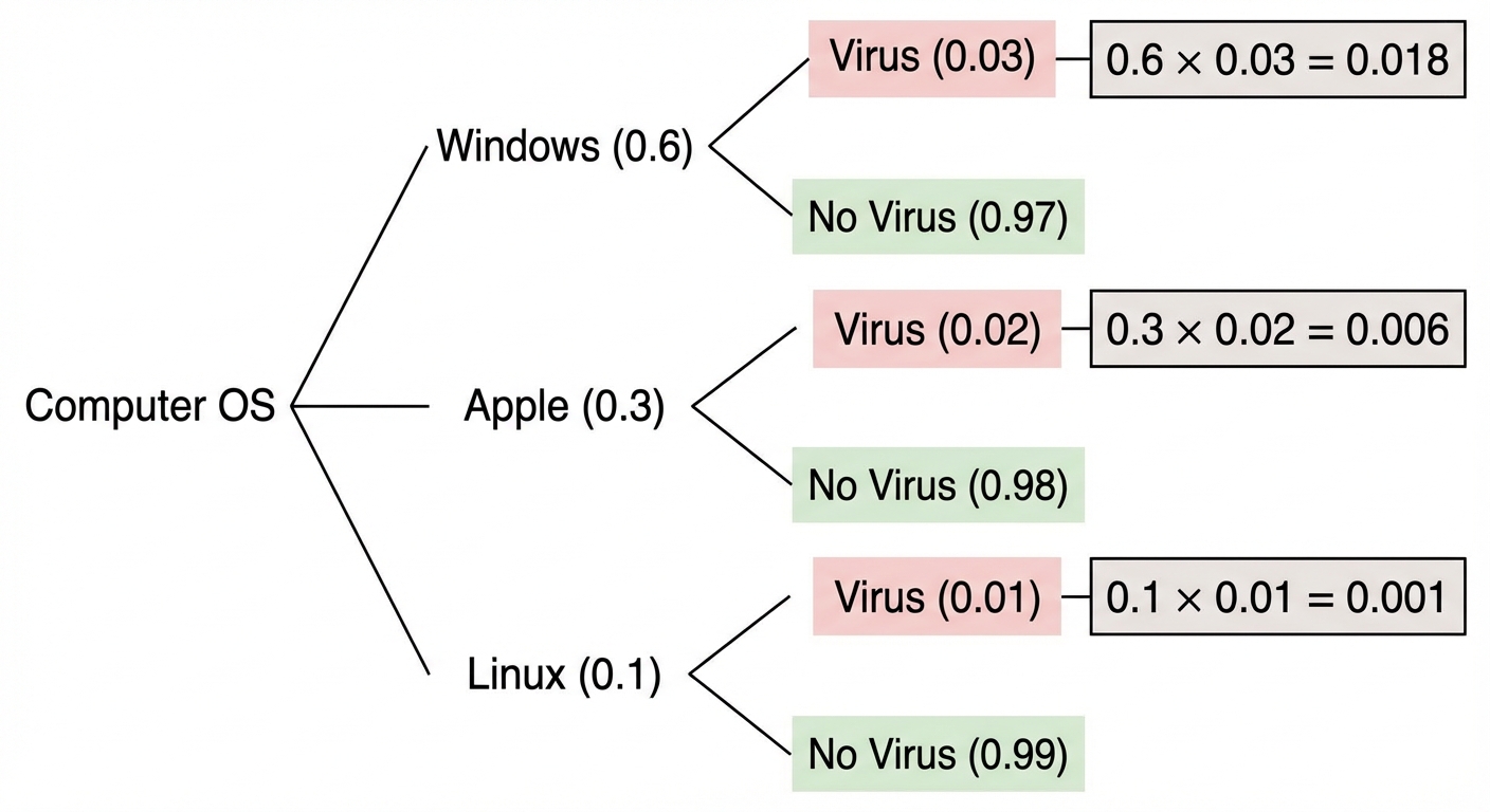
➥ Example 4.3: Computer Virus
- Given: Windows (60%), Apple (30%), Linux (10%).
- Virus Rates: Windows (3%), Apple (2%), Linux (1%).
- Question: What is the probability a randomly selected computer has the virus?
Solution:
P(Virus) = P(W \cap V) + P(A \cap V) + P(L \cap V)
= (0.60)(0.03) + (0.30)(0.02) + (0.10)(0.01)
= 0.018 + 0.006 + 0.001 = 0.025
There is a 2.5% chance a computer has the virus.
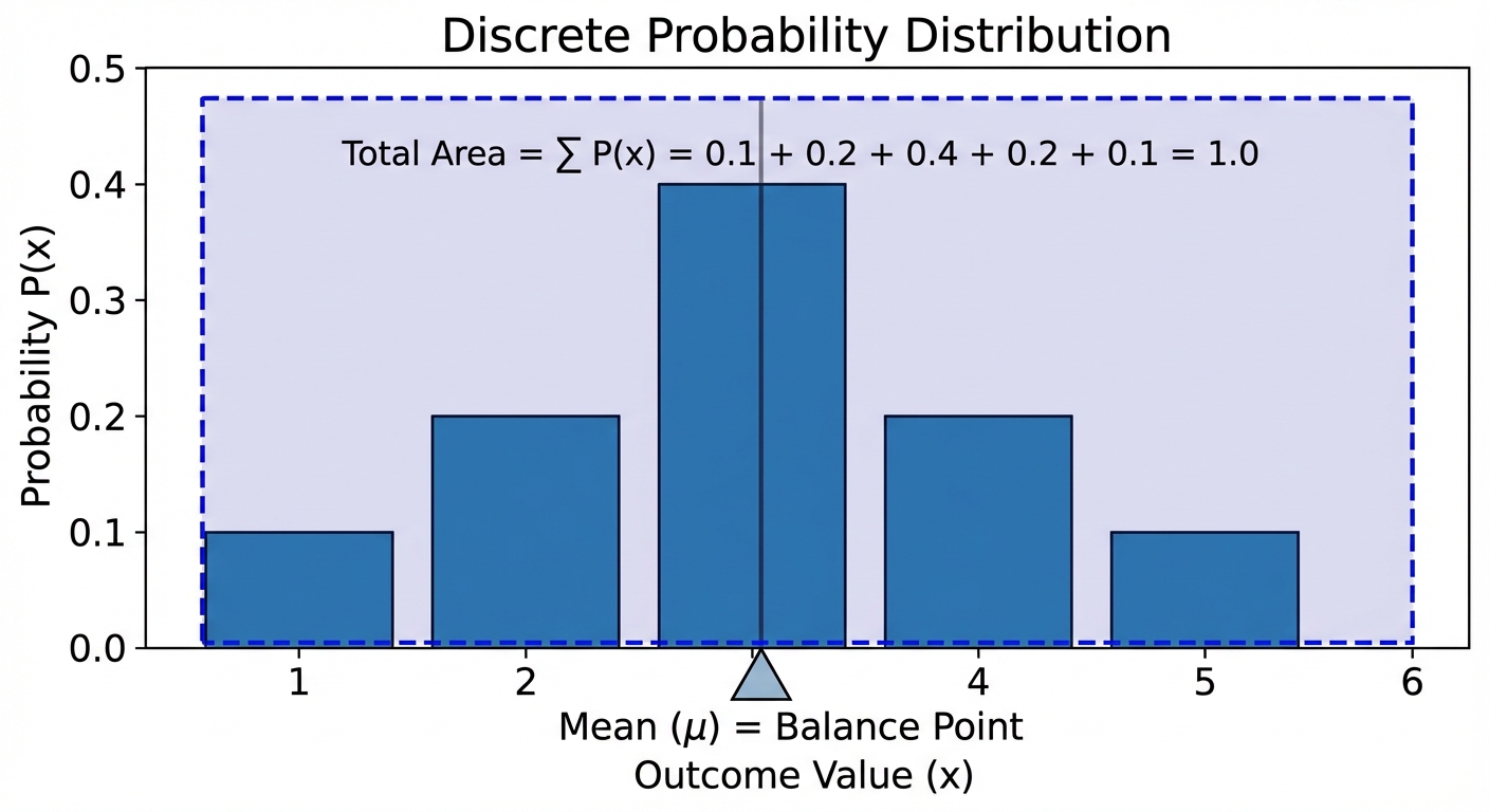
Discrete Random Variables
A Random Variable ($X$) takes numerical values that describe the outcomes of some chance process. A Discrete random variable has a countable number of possible probabilities (gaps between values).
Expected Value (Mean)
The mean of a discrete random variable, $\mu_X$, is the weighted average of all possible values.
\muX = \sum (xi \cdot p_i)
Variance and Standard Deviation
Measures the typical distance of outcomes from the mean.
Variance: $\sigmaX ^2 = \sum (xi - \muX)^2 \cdot pi$
Standard Deviation: $\sigma_X = \sqrt{\text{Variance}}$
➥ Example 4.4: The Lottery Ticket
- 10,000 tickets sold at $1 each.
- Prize: $7,500 (One winner).
- Question: Expected value for a ticket holder?
Setup Table:
| Outcome | Net Gain ($X$) | Probability $P(x)$ |
|---|---|---|
| Win | $7,499 ($7500 - $1 cost) | $1/10,000 = 0.0001$ |
| Lose | -$1 | $9,999/10,000 = 0.9999$ |
Calculation:
\mu_X = (7499)(0.0001) + (-1)(0.9999) = 0.7499 - 0.9999 = -0.25
Interpretation: On average, for every ticket purchased, the buyer expects to lose $0.25.
Combining and Transforming Random Variables
1. Linear Transformations
If we transform reasonable variable $X$ by the equation $Y = a + bX$:
- Mean: Changes with both addition and multiplication.
\muY = a + b\muX - Standard Deviation: Changes only with multiplication (scaling). Adding a constant shifts the graph but does not change the spread.
\sigmaY = |b|\sigmaX
➥ Example 4.8 Refined
Game payoff $X$: Mean $\mu=3.5$, SD $\sigma=2.87$.
A fee of $1 is charged to play, and winnings are doubled. New equation: $Y = 2X - 1$.
- New Mean: $2(3.5) - 1 = 6$.
- New SD: $2(2.87) = 5.74$ (The "-1" has no effect on spread).
2. Sums and Differences of Random Variables
When we combine two random variables $X$ and $Y$:
Mean (Always Add/Subtract):
- $\mu{X+Y} = \muX + \mu_Y$
- $\mu{X-Y} = \muX - \mu_Y$
Variance (ADD ONLY if Independent):
This is the most critical rule. You never add Standard Deviations. You must square them to get variances, add the variances, and root the result.- Condition: $X$ and $Y$ must be INDEPENDENT.
- $\sigma{X+Y}^2 = \sigmaX^2 + \sigma_Y^2$
- $\sigma{X-Y}^2 = \sigmaX^2 + \sigma_Y^2$ (Notice: still addition! Variation always increases when you combine uncertain quantities, even if you subtract the means.)
➥ Example 4.7: Insurance Policies
- Auto Policies ($A$): $\muA = 1.3$, $\sigmaA = 0.9$.
- Home Policies ($H$): $\muH = 0.7$, $\sigmaH = 0.78$.
- Assume Independence (Buying auto does not influence buying home).
Total Policies ($T = A + H$):
- $\mu_T = 1.3 + 0.7 = 2.0$
- $\sigma_T = \sqrt{0.9^2 + 0.78^2} = \sqrt{0.81 + 0.6084} = \sqrt{1.4184} \approx 1.19$
Likely Error Warnng: Do not calculate $0.9 + 0.78 = 1.68$. That is incorrect.
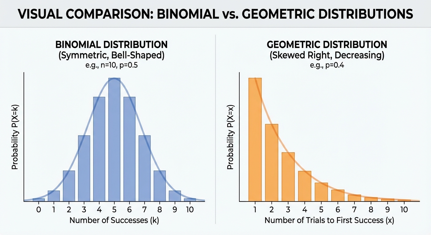
The Binomial Distribution
Used for counting the number of successes in a fixed number of trials.
Conditions (BINS Acronym)
- Binary: Outcomes are Success/Failure.
- Independent: Trials must not influence each other.
- Number: Fixed number of trials ($n$).
- Success: Probability of success ($p$) is constant.
Formulas
If $X$ is Binomial($n, p$):
- Probability: P(X=k) = \binom{n}{k} p^k (1-p)^{n-k}
- Mean: $\mu_X = np$
- Standard Deviation: $\sigma_X = \sqrt{np(1-p)}$
➥ Example 4.9: Defective Bulbs
$p = 0.1$ (defective), $n = 8$.
- P(Exactly 3 defective):
- Formula: $\binom{8}{3} (0.1)^3 (0.9)^5$
- Calculator:
binompdf(n=8, p=0.1, x=3)$\approx 0.033$.
The Geometric Distribution
Used for finding the trial number of the first success. There is no fixed number of trials.
Conditions (BITS Acronym)
- Binary: Outcomes are Success/Failure.
- Independent: Trials are independent.
- Trials: Note the goal is counting trials until the first success.
- Success: Probability of success ($p$) is constant.
Formulas
If $Y$ is Geometric($p$):
- Probability that first success is on trial $k$:
P(Y=k) = (1-p)^{k-1}p - Mean (Expected Wait Time):
\mu_Y = \frac{1}{p} - Standard Deviation:
\sigma_Y = \frac{\sqrt{1-p}}{p}$$
➥ Example 4.10: Ancient Greece
Honesty rate $p=0.12$. We want to meet an honest man.
- Probability 1st honest man is the 3rd person met ($X=3$):
- Formula: Failure, Failure, Success $\rightarrow (0.88)^2 (0.12) = 0.0929$.
- Calculator:
geometpdf(p=0.12, x=3)
- Probability 1st honest man is within the first 4 people ($X \le 4$):
- Calculator:
geometcdf(p=0.12, x=4)$\approx 0.4003$.
- Calculator:
Common Mistakes & Pitfalls
- Independence vs. Mutually Exclusive: Students often think these are synonyms. They are opposites. If two events are mutually exclusive (can't happen together), they are dependent (because if one happens, the probability of the other drops to 0).
- Adding Standard Deviations: Never add $\sigma$. You must variances ($ \sigma^2 $) together to get $\sigma^2_{total}$, then take the square root.
- Binomial vs. Geometric:
- Fixed $n$ trials? $\to$ Binomial.
- "How many trials until…"? $\to$ Geometric.
- Notation: Don't just write calculator speak (
binompdf(8, 0.1, 3)). You must define parameters: "Binomial distribution with $n=8$ and $p=0.1$, seeking $P(X=3)$."