AP Statistics: Binomial and Geometric Random Variables
The Binomial Setting
Not all counts of data are created equal. In AP Statistics, one of the most common discrete random variables you will encounter is the Binomial Random Variable. This specifies a count of "successes" in a fixed number of trials.
Conditions: The BINS Acronym
To verify that a random variable is binomial, you must strictly ensure it meets the BINS conditions:
- B - Binary: The possible outcomes of each trial can be classified as "Success" or "Failure."
- I - Independent: Trials must be independent; knowing the result of one trial must not tell you anything about the result of the next.
- N - Number: The number of trials, typically denoted as $n$, must be fixed in advance.
- S - Success: The probability of success, denoted as $p$, must be the same for each trial.
Note on the 10% Condition: Strictly speaking, sampling without replacement violates the "Independent" condition because probabilities change slightly as you remove items. However, if the sample size $n$ is less than 10% of the population size ($N$), we can treat the trials as independent for calculation purposes.
Binomial Probability Formula
If $X$ is a binomial random variable with parameters $n$ and $p$, the probability of getting exactly $k$ successes is:
Where:
- $\binom{n}{k}$ is the binomial coefficient (read as "n choose k"), calculated as $\frac{n!}{k!(n-k)!}$. This counts the number of ways to arrange $k$ successes among $n$ trials.
- $p^k$ represents the probability of the $k$ successes.
- $(1-p)^{n-k}$ represents the probability of the remaining failures.
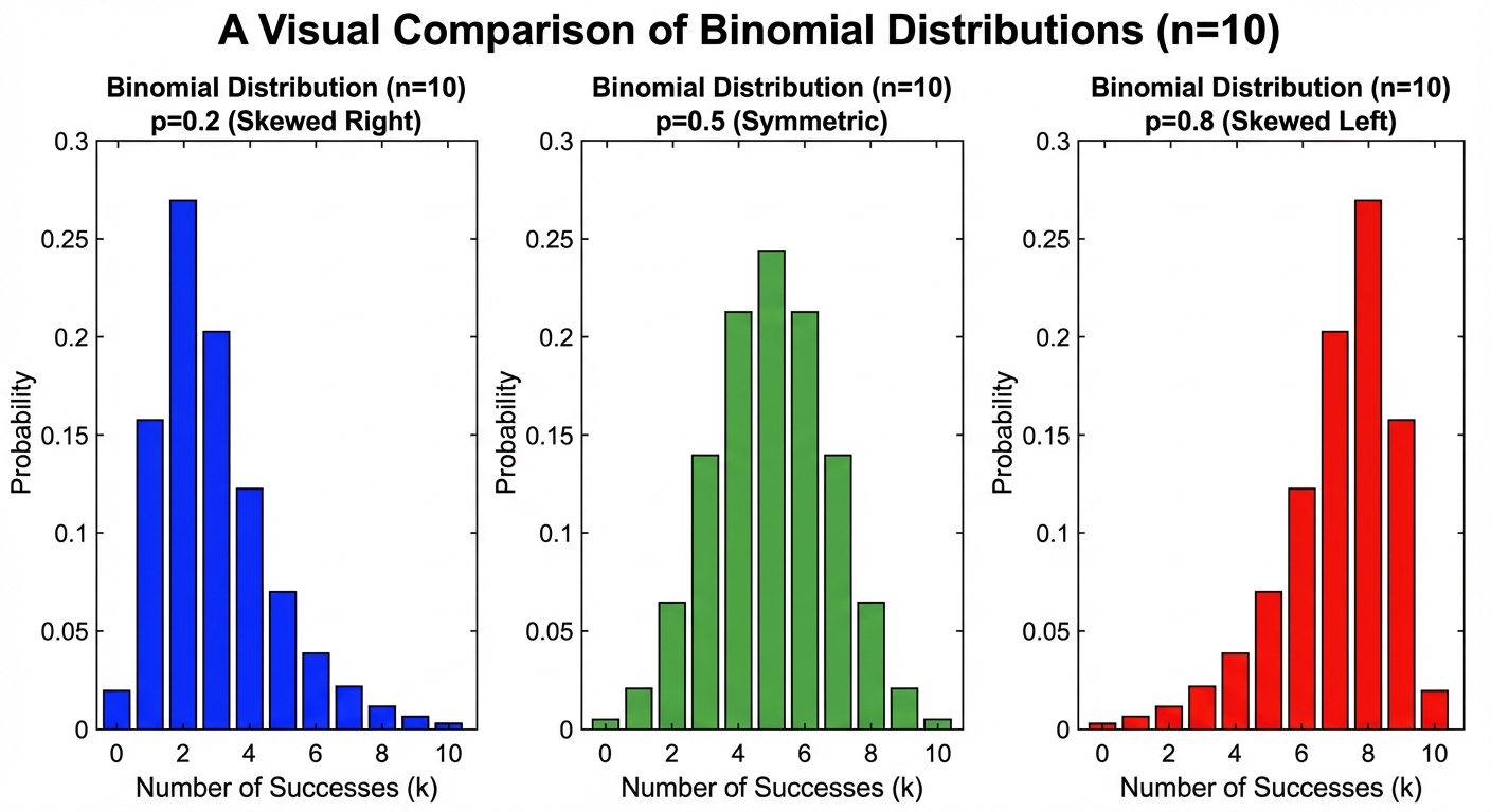
Describing the Distribution: Center and Spread
The shape of a binomial distribution depends on $p$. If $p = 0.5$, it is symmetric. If $p < 0.5$, it is skewed right. If $p > 0.5$, it is skewed left.
We determine the center and spread using these formulas (these are on the AP Formula Sheet):
| Parameter | Formula |
|---|---|
| Mean (Expected Value) | $\mu_X = np$ |
| Standard Deviation | $\sigma_X = \sqrt{np(1-p)}$ |
The Large Counts Condition
Can we approximate a Binomial distribution using a Normal Distribution? Yes, but only if the expected number of successes and failures are both sufficiently large. This is tested using the Large Counts Condition:
- $np \geq 10$
- $n(1-p) \geq 10$
If both are true, the distribution is approximately Normal: $N(np, \sqrt{np(1-p)})$.
The Geometric Setting
While the Binomial distribution counts successes in a fixed number of trials, the Geometric Distribution counts the number of trials required to achieve the first success.
Conditions: BIN vs. BINS
The conditions are almost identical to Binomial, with one crucial difference regarding the "Number" of trials:
- Binary: Outcomes are Success/Failure.
- Independent: Trials are independent.
- Trials until Success: We do not have a fixed $n$. We flip the coin (or take the shot) until we get a success.
- Success: Probability $p$ is constant.
Geometric Probability Formula
If $Y$ is a geometric random variable with probability of success $p$, the probability that the first success occurs on the $k$-th trial is:
Logic: You must fail $k-1$ times (probability $1-p$ each time) and then succeed once (probability $p$) at the very end.
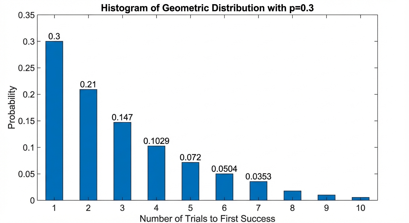
Describing the Distribution
Unlike Binomial distributions, which can be symmetric, Geometric distributions are ALWAYS skewed right. The most likely outcome is always that the success happens on the 1st trial ($k=1$), and probabilities decrease as $k$ increases.
| Parameter | Formula |
|---|---|
| Mean (Expected Value) | $\mu_Y = \frac{1}{p}$ |
| Standard Deviation | $\sigma_Y = \frac{\sqrt{1-p}}{p}$ |
Example: If you are a 20% free throw shooter ($p=0.2$), how many shots do you expect to take to make one? $\mu = 1/0.2 = 5$ shots.
Calculator Functions & CDFs
In AP Statistics, you will likely use a graphing calculator (like the TI-84) to compute probabilities. It is vital to distinguish between PDF and CDF.
PDF vs. CDF
- PDF (Probability Density/Mass Function): Calculates the probability of an exact value. e.g., $P(X = 3)$.
- CDF (Cumulative Distribution Function): Calculates the accumulated probability from 0 up to a value. e.g., $P(X \leq 3)$.
| Concept | TI-84 Function | Used For |
|---|---|---|
| Binomial Exact | binompdf(n, p, k) | $P(X = k)$ |
| Binomial Cumulative | binomcdf(n, p, k) | $P(X \le k)$ |
| Geometric Exact | geometpdf(p, k) | $P(Y = k)$ |
| Geometric Cumulative | geometcdf(p, k) | $P(Y \le k)$ |
Warning: The calculator only sums from the left (lower tail). If you need $P(X \geq 3)$ (at least 3), you must use the complement rule: $1 - P(X \le 2)$.
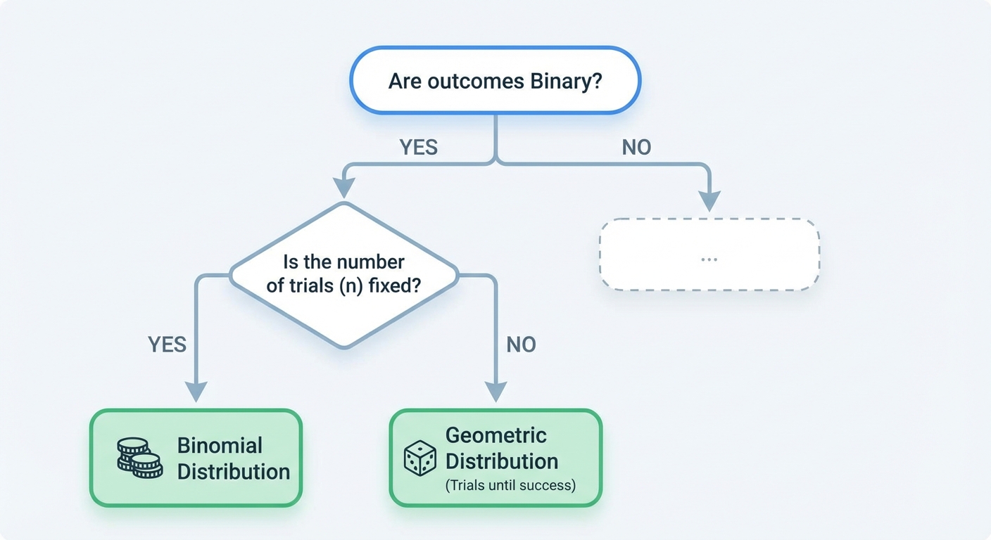
Comparison and Decision Making
When you see a word problem, how do you know which distribution to use?
Worked Example: Binomial
Scenario: A basketball player makes 80% of her free throws. She takes 10 shots.
- Check BINS: Binary (Make/Miss), Independent (assumed), Number fixed ($n=10$), Success constant ($p=0.8$). It is Binomial.
- Question: What is the probability she makes exactly 8?
- Calculation: $P(X=8) = \binom{10}{8}(0.8)^8(0.2)^2 \approx 0.302$.
Worked Example: Geometric
Scenario: The same player keeps shooting until she misses (to test her consistency). A "success" here is defined as a "miss" for the sake of the math ($p=0.2$).
- Check: Binary, Independent, Until success. It is Geometric.
- Question: What is the probability the first miss comes on the 4th shot?
- Calculation: $P(Y=4) = (1-0.2)^{3}(0.2) = (0.8)^3(0.2) = 0.1024$.
Common Mistakes & Pitfalls
Confusing "At Least" and "At Most"
- "At most 5" means $X \le 5$ (use
binomcdfdirectly). - "At least 5" means $X \ge 5$. Calculators don't do this directly. You must calculate $1 - P(X \le 4)$.
- "At most 5" means $X \le 5$ (use
Forgetting to define the variable
- On the FRQ (Free Response Question), do not just write "binompdf(10, 0.5, 3)". This is "calculator speak" and receives no credit for communication. You must write: "Let $X$ be the number of heads. $X \sim B(10, 0.5)$. We want $P(X=3)$."
Geometric Definitions
- Remember that the geometric variable $X$ is the number of trials, not the number of failures. If the first success is on the 3rd trial, $X=3$ (Failure, Failure, Success). Variations exist where $X$ counts failures, but in AP stats, $X$ usually counts trials including the success.
Misidentifying Non-Independent Events
- If you draw cards from a deck without replacement, $p$ changes slightly with every draw. This is Hypergeometric, not Binomial. However, if the deck is massive (10% condition), we approximate as Binomial.