Comprehensive Guide to Hypothesis Testing for Means
Significance Test for a Population Mean
When we want to test a claim about an unknown population mean ($ \mu $) using a sample mean ($ \bar{x} $), we use a One-Sample t-Test.
Because we rarely know the true population standard deviation ($ \sigma $), we substitute it with the sample standard deviation ($ s $). This introduces extra uncertainty, requiring the use of the t-distribution (which has heavier tails than the Normal distribution) rather than the z-distribution.
Conditions for Inference
Before calculating, you must verify the "SIN" conditions:
- Sample (Random): The data must come from a randomized experiment or a random sample.
- Independence (10% Condition): If sampling without replacement, the sample size ($ n $) must be less than 10% of the population size ($ N $). ($ n \le 0.10N $).
- Normal/Large Sample: Determine if the sampling distribution of $ \bar{x} $ is approximate normal:
- If the population is known to be Normal, you are good.
- Central Limit Theorem (CLT): If $ n \ge 30 $, the sampling distribution is approximately normal.
- If $ n < 30 $, plot the data (dot plot or boxplot). If there is no strong skewness or outliers, you can proceed with caution.
The t-Distribution and Degrees of Freedom
The shape of the t-distribution depends on the Degrees of Freedom (df).
As $ n $ increases, the t-distribution approaches the Standard Normal ($ z $) distribution.
Test Statistic Formula
The t-statistic measures how many standard errors the sample mean is away from the hypothesized mean ($ \mu_0 $).
Where:
- $ \bar{x} $ = Sample mean
- $ \mu0 $ = Hypothesized population mean (from $ H0 $)
- $ s $ = Sample standard deviation
- $ n $ = Sample size
- $ \frac{s}{\sqrt{n}} $ = Standard Error of the mean ($ SE_{\bar{x}} $)
Worked Example: One-Sample t-Test
Scenario: A coffee shop claims their medium coffee contains 12 oz. You suspect they are underfilling cups. You sample 15 cups randomly; the mean is 11.8 oz with a standard deviation of 0.4 oz. A dot plot shows no strong skew.
- Hypotheses:
- $ H_0: \mu = 12 $
- $ H_a: \mu < 12 $ (One-sided)
- Conditions: Random (stated), 10% (safe to assume >150 cups sold), Normal (Graph check passed, $ n < 30 $).
- Math:
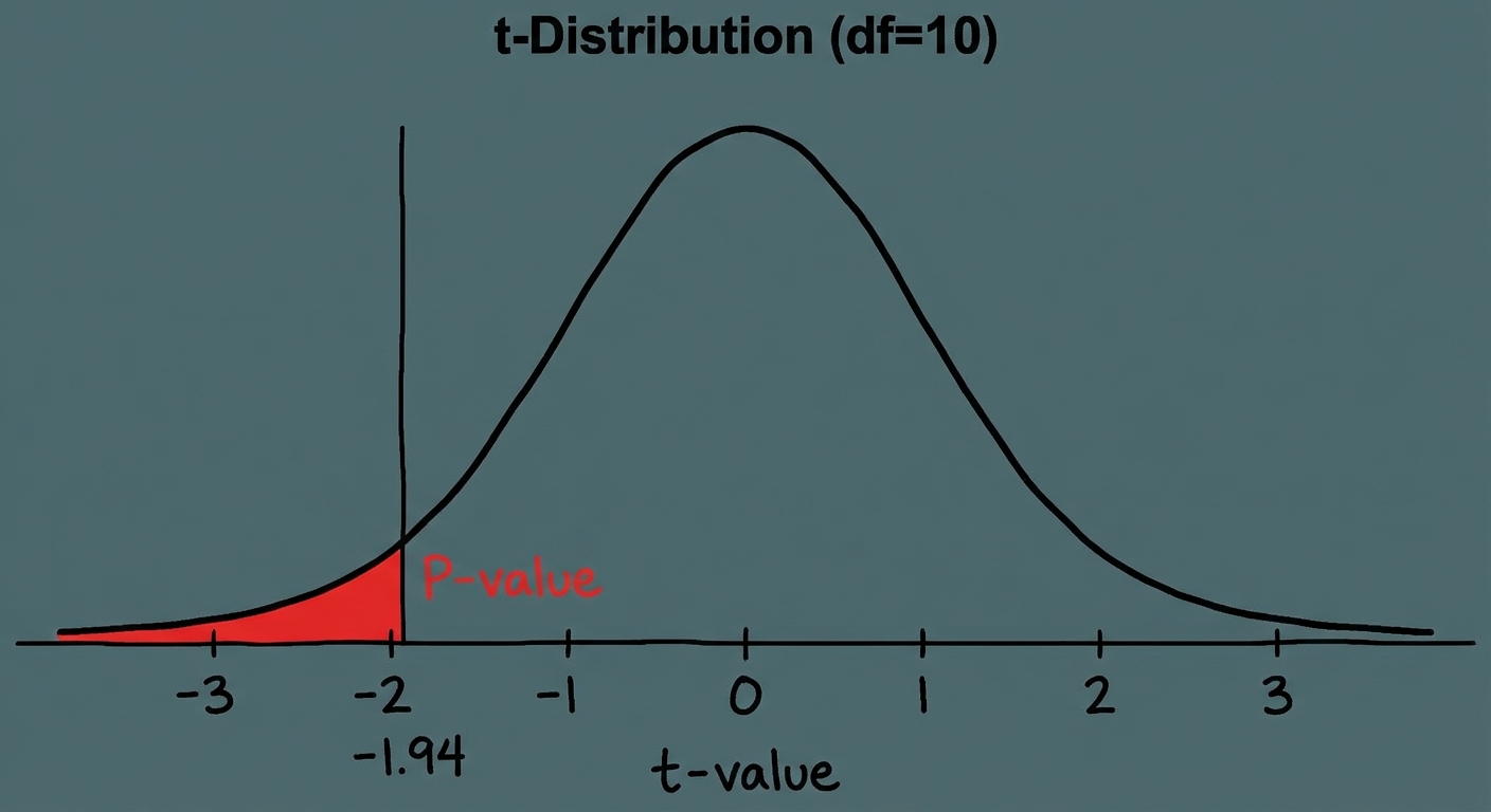
- P-Value: Using a t-table or calculator
tcdf(-1E99, -1.94, 14), $ p \approx 0.036 $. - Conclusion: Since $ p $ (0.036) $ < \alpha $ (0.05), we reject $ H_0 $. There is convincing evidence the true mean volume is less than 12 oz.
Matched Pairs t-Test
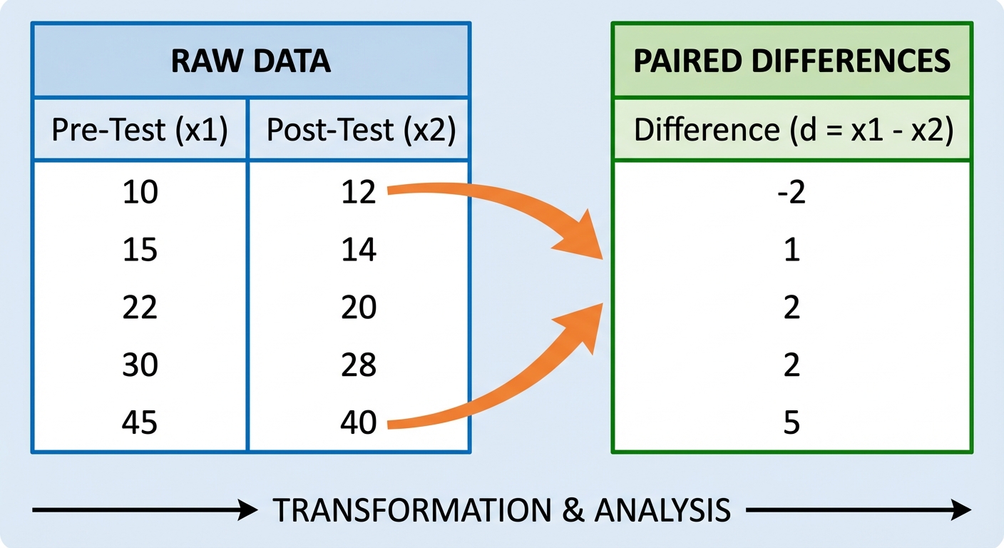
This is a specific type of One-Sample t-Test applied when data is paired or dependent. We do not compare two separate means; we analyze the mean of the differences.
Identifying Matched Pairs
Use this test when:
- Pre-test/Post-test: One subject measured twice.
- Matching Subjects: Twins, siblings, or partners paired together.
- Cross-over Design: One subject tries Treatment A, then Treatment B.
The variable of interest is $ \mu_d $ (the true mean difference).
Hypotheses
The null hypothesis usually states there is no difference.
- $ H0: \mud = 0 $
- $ Ha: \mud \neq 0 $ (or $ < 0 $, $ > 0 $)
Formula
We treat the list of differences as a single sample.
- $ \bar{x}_{diff} $: The mean of the differences.
- $ s_{diff} $: The standard deviation of the differences.
- $ n_{pairs} $: The number of pairs (not total observations).
Significance Test for the Difference of Two Means
Use the Two-Sample t-Test when comparing means from two independent groups (e.g., Men vs. Women, Control Group vs. Experimental Group).
Hypotheses
- $ H0: \mu1 - \mu2 = 0 $ (or $ \mu1 = \mu_2 $)
- $ Ha: \mu1 - \mu_2 \neq 0 $ (or $ < $, $ > $)
Conditions
Crucially, the groups must be independent of each other.
- Random: Both samples are random (or randomized allocation).
- 10% Rule: Applies to both populations independently (if sampling without replacement).
- Normal/Large: $ n1 \ge 30 $ AND $ n2 \ge 30 $, or check graphs for both samples.
Standard Error & Test Statistic
Variances add, standard deviations do not. Therefore, the standard error involves adding the variances of both samples.
Usually, $ (\mu1 - \mu2)_0 = 0 $, so the numerator simplifies to just the difference in sample means.
Degrees of Freedom
There are two ways to calculate df for two-sample t-tests:
- Calculator Measure (Preferred): The Satterthwaite approximation (a complex formula usually yielding a decimal df). This is more powerful and accurate.
- Conservative Estimate: $ df = \text{min}(n1 - 1, n2 - 1) $.
Note for AP Exam: Always use the calculator result if available; use the conservative method only if calculating by hand without technology.
To Pool or Not to Pool?
Do NOT Pool. In AP Statistics, we generally assume equal variances are unknown and likely unequal. Only pool variances if specifically told the population variances are equal (rare). Use unpooled t-procedures.
Summary of Notations
| Concept | One-Sample | Matched Pairs | Two-Sample |
|---|---|---|---|
| Parameter | $ \mu $ | $ \mu_d $ | $ \mu1 - \mu2 $ |
| Statistic | $ \bar{x} $ | $ \bar{x}_{diff} $ | $ \bar{x}1 - \bar{x}2 $ |
| Sample Size | $ n $ | $ n $ (pairs) | $ n1 $ and $ n2 $ |
| DoF | $ n-1 $ | $ n-1 $ | Calculator or $ \min(n1-1, n2-1) $ |
Mnemonics
Use PHANTOMS to structure your Free Response Answer:
- Parameter (Define $ \mu $ in context)
- Hypotheses (State $ H0, Ha $)
- Assumptions (Check SIN conditions)
- Name the test (e.g., "Two-Sample t-Test")
- Test Statistic (Calculate $ t $)
- Obtain P-value (Draw curve, find area)
- Make Decision (Reject or Fail to Reject based on $ \alpha $)
- State Conclusion (In context)
Common Mistakes & Pitfalls
Confusing Matched Pairs with Two-Sample t-tests:
- The Trap: Seeing two columns of numbers and automatically assuming Two-Sample t-test.
- The Fix: Ask: "Are these two separate groups of people, or the same people measured twice?" If the data is linked row-by-row, it is Paired.
Using $ z $ instead of $ t $:
- The Trap: Using Inverse Norm or NormalCDF for means.
- The Fix: If you are using $ s $ (sample SD) instead of $ \sigma $ (population SD), you MUST use $ t $.
Sloppy Condition Checking:
- The Trap: Writing "$ n \ge 30 $" when $ n=15 $.
- The Fix: If $ n < 30 $, you must explicitly mention looking at a graph for skewness/outliers. You cannot just say "sample is large enough."
Accepting the Null:
- The Trap: Concluding "We accept $ H_0 $."
- The Fix: We never prove the Null. We only "Fail to reject $ H_0 $." (Think of a court trial: "Not Guilty" does not mean "Innocent," it just means insufficient evidence of guilt).