Comprehensive Guide to Data Analysis and Statistics
Unit 1: Exploring One-Variable Data
Introduction to Data Variables
Statistics is the science of learning from data. To analyze data effectively, we must first classify the type of variables we are measuring.
Categorical vs. Quantitative Variables
Categorical (Qualitative) Variables
- Definition: Places an individual into one of several groups or categories.
- Values: Labels, names, or non-numerical descriptions (e.g., Eye Color, Zip Code, Grade Level).
- Visualization: Bar charts, Pie charts.
- Summary: Counts (frequencies) and Proportions (relative frequencies).
Quantitative Variables
- Definition: Takes numerical values for which arithmetic operations (like adding or averaging) make sense.
- Values: Counts or measurements.
- Types:
- Discrete: Takes a fixed set of countable values with gaps between them (e.g., Number of siblings, Shoe size).
- Continuous: Takes any value in an interval with no gaps (e.g., Height, Weight, Time to run a mile).
Categorical Data: Frequency and Relative Frequency
Data is often summarized in tables before graphing.
- Frequency Table: Displays the count (number of individuals) in each category.
- Relative Frequency Table: Displays the percent or proportion of individuals in each category.
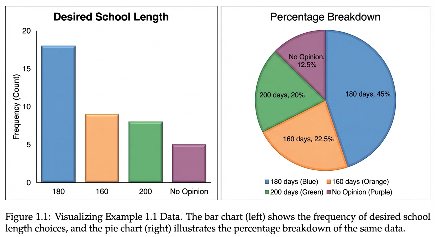
➥ Example 1.1: School Year Length Survey
A survey asked 2,000 parents about their preferred school year length.
| Preference | Frequency | Relative Frequency | Calculation |
|---|---|---|---|
| 180 Days | 1100 | 0.55 | $1100/2000$ |
| 160 Days | 300 | 0.15 | $300/2000$ |
| 200 Days | 500 | 0.25 | $500/2000$ |
| No Opinion | 100 | 0.05 | $100/2000$ |
| Total | 2000 | 1.00 |
Visualizing Categorical Data
- Bar Chart: Bars represent categories; height represents frequency/relative frequency. Bars should not touch.
- Pie Chart: Slices represent the proportion of the whole. Useful only when categories sum to 100%.
Visualizing Quantitative Data
When we graph quantitative data, we look for visual patterns. The three most common basics are Dotplots, Stemplots, and Histograms.
1. Dotplots
Each data value is shown as a dot above its location on a number line.
- Pros: Shows every individual data value; easy to make for small datasets.
- Cons: Becomes cluttered with large datasets.
2. Stemplots (Stem-and-Leaf Plots)
A simple graphical display for fairly small data sets.
- Stem: The first digit(s) of the number.
- Leaf: The final digit. Leaves must be single digits.
- Mandatory: You must include a KEY interpreting the stem and leaf (e.g., "Key: 4|2 means 42 years old").
- Split Stems: If data is clumped, you can split stems (e.g., 10-14 on the first '1' stem, 15-19 on the second '1' stem).
3. Histograms
A graph for large quantitative datasets.
- Divide the data into classes (bins) of equal width.
- Count the frequency (or relative frequency) in each bin.
- Draw bars where height = frequency. Bars must touch (unlike bar charts) to indicate continuous data.
➥ Example 1.2: AP Classes Taken
Data from 2,200 seniors regarding how many AP classes they take:
| AP Classes | Frequency | Rel. Freq |
|---|---|---|
| 0 | 400 | 0.18 |
| 1 | 500 | 0.23 |
| 2 | 900 | 0.41 |
| 3 | 300 | 0.14 |
| 4 | 100 | 0.05 |
Note: The shape of the histogram remains the same whether the vertical axis is Frequency or Relative Frequency.
Describing Distributions (The SOCS Method)
When asked to "describe the distribution" of a quantitative variable on the AP exam, you must address four key characteristics. Use the acronym SOCS.
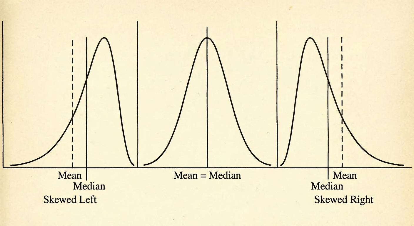
1. Shape (S)
Describe the overall pattern of the graph.
- Symmetric: Left and right sides are approximate mirror images.
- Skewed Right (Positively Skewed): Tail extends to the right (higher values). Mean > Median.
- Skewed Left (Negatively Skewed): Tail extends to the left (lower values). Mean < Median.
- Modes:
- Unimodal: One distinct peak.
- Bimodal: Two distinct peaks (often suggests two different populations, e.g., men's and women's heights).
- Uniform: Roughly flat; no distinct peak.
2. Outliers (O)
Mention any unusual features.
- Outliers: Values that fall far away from the rest of the data.
- Gaps: Large spaces between data points.
- Clusters: Distinct groups of data.
3. Center (C)
A single value that describes the middle of the distribution.
- Median: The midpoint.
- Mean: The arithmetic average.
4. Spread (S)
How variable is the data? (Also called dispersion or variability).
- Range: Max - Min (a single number, not an interval).
- IQR: Interquartile Range.
- Standard Deviation: Average distance from the mean.
Summary Statistics
Measuring Center
The Mean ($\bar{x}$)
The arithmetic average. Used for symmetric distributions without outliers.
The Median ($M$)
The midpoint of a distribution. Half the observations are smaller, half are larger.
- Order numbers from smallest to largest.
- If $n$ is odd, the median is the center number.
- If $n$ is even, the median is the average of the two center numbers.
Resistance (Key Concept)
- Resistant Measures: Median and IQR. Extreme values (outliers) or strong skew do not affect them significantly.
- Non-Resistant Measures: Mean and Standard Deviation. One large outlier can pull the mean toward it significantly.
Rule of Thumb: Use Median/IQR for skewed data. Use Mean/SD for symmetric data.
Measuring Spread (Variability)
1. Range
- Weakness: Extremely sensitive to outliers.
2. Standard Deviation ($s_x$)
Measures the "typical" distance of the values from the mean.
- $sx = \sqrt{\frac{\sum(xi - \bar{x})^2}{n-1}}$
- Interpretation: "On average, [variable name] varies by [SD value] units from the mean."
- Variance ($s^2$): The standard deviation squared.
3. Interquartile Range (IQR)
The range of the middle 50% of the data.
- Q1 (First Quartile): Median of the lower half of data.
- Q3 (Third Quartile): Median of the upper half of data.
➥ Example 1.6: Teacher Ages
Consider ages: {24, 25, 25, 29, 34, 37, 41, 42, 48, 48, 54, 61}. ($n=12$)
- Mean: $\bar{x} = 39$ years.
- Finding Quartiles:
- Split data: Lower {24…37}, Upper {41…61}.
- $Q_1 = \frac{25+29}{2} = 27$
- $Q_3 = \frac{48+48}{2} = 48$
- IQR $= 48 - 27 = 21$ years.
- Standard Deviation: $s_x \approx 11.66$ years.
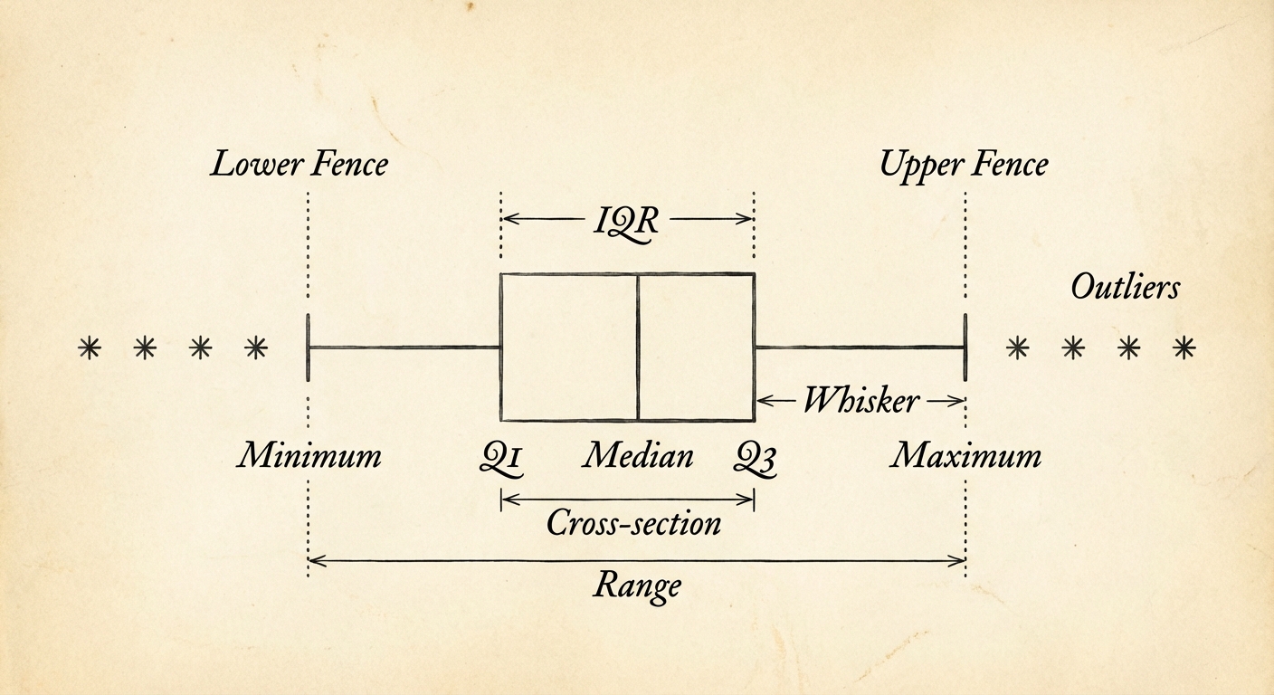
Boxplots and Outliers
Five-Number Summary
A distribution is summarized by: Min, Q1, Median, Q3, Max.
The 1.5 $\times$ IQR Rule for Outliers
An observation is mathematically an outlier if it falls outside the "fences":
- Lower Fence: $Q_1 - 1.5(IQR)$
- Upper Fence: $Q_3 + 1.5(IQR)$
Constructing a Boxplot
- Calculate 5-number summary and Fences.
- Draw a central box from $Q1$ to $Q3$. Mark the Median inside the box.
- Whiskers: Extend lines from the box to the smallest and largest observations that are NOT outliers (do not extend to the fences!).
- Outliers: Mark any data points outside the fences as distinct dots or asterisks.
Comparing Distributions
When comparing distributions (e.g., parallel boxplots, back-to-back stemplots), you strictly typically follow the SOCS method, using comparative language (greater than, less than, similar to).
➥ Example 1.9: NBA Wins (East vs. West)
- Shape: The East is roughly symmetric, while the West is roughly uniform.
- Center: The median wins for the West (49) is greater than the median for the East (41).
- Spread: The East has a larger range (43) compared to the West (38).
- Variability: The West has a specific outlier at 19 wins, whereas the East has no outliers.
Cumulative Relative Frequency Graphs (Ogives)
These graphs display the percentile of a distribution.
- X-axis: Variable value.
- Y-axis: Cumulative Relative Frequency (0 to 1, or 0% to 100%).
- Interpretation: A point at $(x, y)$ means $y$% of the data is less than or equal to $x$.
The Normal Distribution
A specific type of symmetric, bell-shaped density curve used to model many natural phenomena.
Properties
- Defined by Mean ($\mu$) and Standard Deviation ($\sigma$).
- Mean = Median = Mode (at the center).
- Total area under the curve = 1 (100%).
The Empirical Rule (68-95-99.7)
For a Normal distribution:
- 68% of data falls within $\mu \pm 1\sigma$
- 95% of data falls within $\mu \pm 2\sigma$
- 99.7% of data falls within $\mu \pm 3\sigma$
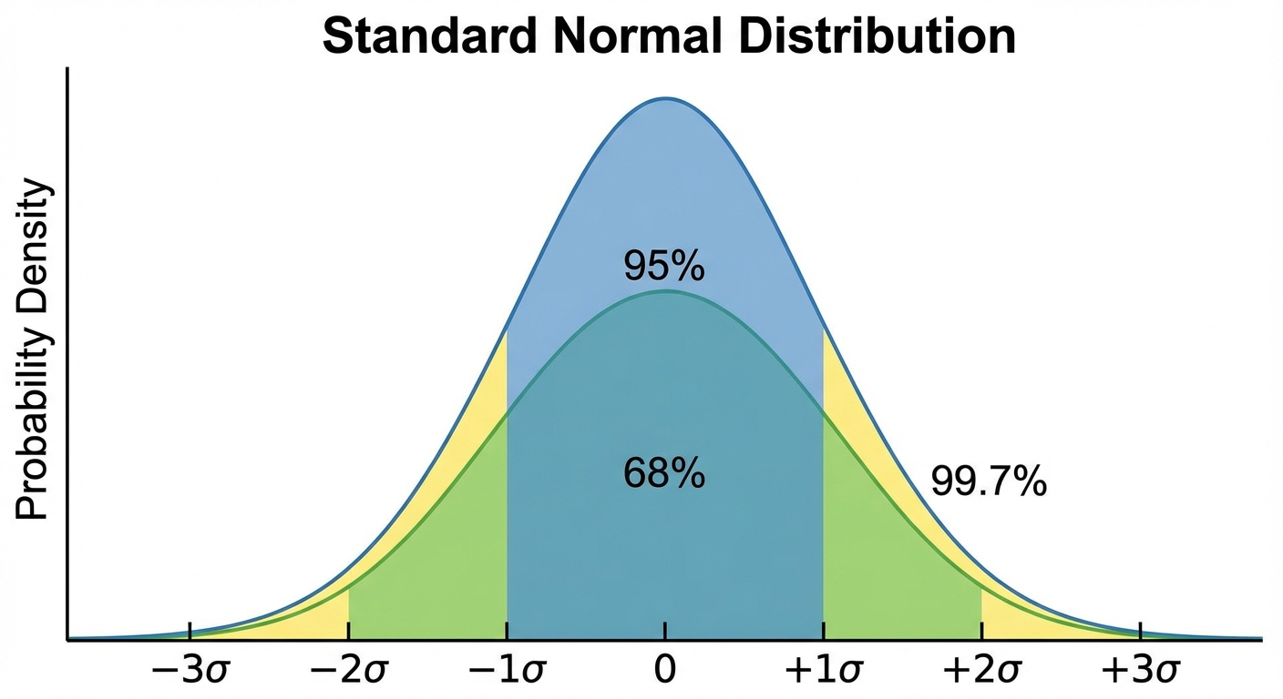
➥ Example 1.13: Taxi Miles
Mean $\mu = 75,000$, SD $\sigma = 12,000$. Normal Distribution.
- 68% of taxis drive between $63,000$ $(75k - 12k)$ and $87,000$ $(75k + 12k)$ miles.
- 95% range: $51,000$ to $99,000$ miles.
Standardizing (z-scores)
To compare values from different distributions, we calculate a z-score. It measures how many standard deviations a value $x$ is from the mean.
- Positive z-score: Value is above the mean.
- Negative z-score: Value is below the mean.
- Context: A z-score of 2.0 or higher is often considered "unusual."
Common Mistakes & Pitfalls
- Thinking Categorical Variables are Quantitative: Just because a variable involves numbers doesn't make it quantitative. Zip codes and Area codes are categorical (they are labels, you can't average them).
- Forgetting Context: Never list numbers for Center or Spread without mentioning the variable name (e.g., "The median height is…").
- Vague Comparisons: When comparing distributions, avoiding saying "The spread is different." You must say "The spread of Group A is larger than Group B."
- Bar Charts vs. Histograms: Bars touch in histograms (continuous data). Bars do not touch in bar charts (categorical).
- Boxplot Whiskers: A common error is drawing whiskers to the "fences." Whiskers must stop at the last actual data point inside the fence.