AP Macro Unit 1: Foundations of Economic Analysis
1. Foundations of Economic Analysis
1.1 Scarcity and Economic Systems
The Fundamental Economic Problem
Economics is the social science that studies how individuals, governments, firms, and nations make choices on allocating scarce resources to satisfy their unlimited wants.
- Scarcity: This is the basic economic problem. It exists because human wants are unlimited, but the resources available to satisfy those wants are limited.
- Note: Scarcity is not the same as poverty; even wealthy nations and individuals face scarcity (e.g., scarcity of time).
Microeconomics vs. Macroeconomics
- Microeconomics: Focuses on individual decision-making units (households, firms) and specific markets (e.g., the market for smartphones).
- Macroeconomics: Focuses on the economy as a whole. It aggregates microeconomic behavior to look at broad indicators like inflation, unemployment, and Gross Domestic Product (GDP).
factors of Production (Resource Categories)
To produce goods and services, an economy needs resources. These are categorized into four groups, often summarized by the acronym CELL:
- Capital (Physical Capital): Human-made resources used to produce other goods.
- Examples: Machinery, factories, robots, computers, tools.
- Important Distinction: In economics, money makes nothing. Money is considered "financial capital," not a productive resource. Changing the money supply affects prices, but printing money does not create more factories.
- Entrepreneurship: The human resource that combines the other factors. Entrepreneurs take risks to earn profits.
- Land: All natural resources found in nature.
- Examples: Water, minerals, timber, oil, arable land.
- Labor: Physical and mental human effort employed in the production process.
1.2 Opportunity Cost and the PPC
Opportunity Cost vs. Trade-Offs
Because of scarcity, every choice implies a cost.
- Trade-off: All the alternatives that we give up whenever we choose one course of action over others.
- Opportunity Cost: The value of the next best specific alternative given up when a choice is made. It is not the sum of all alternatives, just the best one.
The Production Possibilities Curve (PPC)
The PPC is a graphical model that shows the maximum combinations of two goods that can be produced if all resources are fully employed and used efficiently.

Interpreting Points on the PPC
- On the Curve (Points A, B, C): Represents productively efficient use of resources. The economy is maximizing output.
- Inside the Curve (Point D): Represents inefficiency or unemployment. Resources are being wasted or lying idle (e.g., high unemployment rate).
- Outside the Curve (Point E): Currently unattainable given current resources and technology.
Shape of the PPC
- Concave (Bowed Out) to Origin: Indicates Increasing Opportunity Cost.
- Why? Resources are not perfectly adaptable. As you produce more of Good A (e.g., Tanks), you must use resources less suited for it (e.g., bakers), sacrificing increasing amounts of Good B (e.g., Bread).
- Straight Line: Indicates Constant Opportunity Cost.
- Why? Resources are perfectly substitutable between the two goods (e.g., Calzones vs. Pizza).
Shifting the PPC (Economic Growth)
The PPC represents the potential output of an economy. It shifts outward (Economic Growth) if:
- Resource Quantity Increases: More labor relations, new territory, discovered oil.
- Resource Quality Increases: Better education (Human Capital), training.
- Technology: Improved production methods.
- Contraction: The curve shifts inward if resources are destroyed (war, natural disaster).
1.3 Comparative Advantage and Trade
Trade allow countries to consume beyond their own production possibilities curve.
Absolute vs. Comparative Advantage
- Absolute Advantage: The ability to produce more of a good with the same amount of resources (or the same amount with fewer resources).
- Focus: Who is better/faster?
- Comparative Advantage: The ability to produce a good at a lower opportunity cost than another producer.
- Focus: Who gives up less to do it?
- Key Principle: Countries should specialize in what they have a comparative advantage in and trade for the rest.

Calculating Opportunity Cost
There are two types of problems in AP Macro: Output and Input.
1. Output Problems (OOO)
Data shows how much product is created with fixed resources (e.g., "Tons of wheat produced in 1 hour").
- Rule: Output? Other goes Over.
- Equation:
Example:
- Japan: 4 Cars or 2 Trucks
- Opp Cost of 1 Car = $2/4$ = 0.5 Trucks
2. Input Problems (IOU)
Data shows how many resources are required to create one unit of product (e.g., "Hours to bake a cake").
- Rule: Input? Other goes Under.
- Equation:
Example:
- USA: 10 hours for a Car
- Mexico: 2 hours for a Car
- USA has Absolute Disadvantage (slower), but we must check math for Comparative Advantage.
Terms of Trade
For trade to be beneficial, the "price" (exchange rate) of a good must fall between the opportunity costs of the buyer and the seller.
- If Country A produces corn at a cost of 2 wheat, and Country B produces corn at a cost of 4 wheat, a fair trade price for 1 corn is between 2 and 4 wheat.
1.4 Demand
The Law of Demand
There is an inverse relationship between Price ($P$) and Quantity Demanded ($Q_d$).
- As $P \uparrow$, $Q_d \downarrow$
- As $P \downarrow$, $Q_d \uparrow$
This creates a downward-sloping curve.
Change in Quantity Demanded vs. Change in Demand
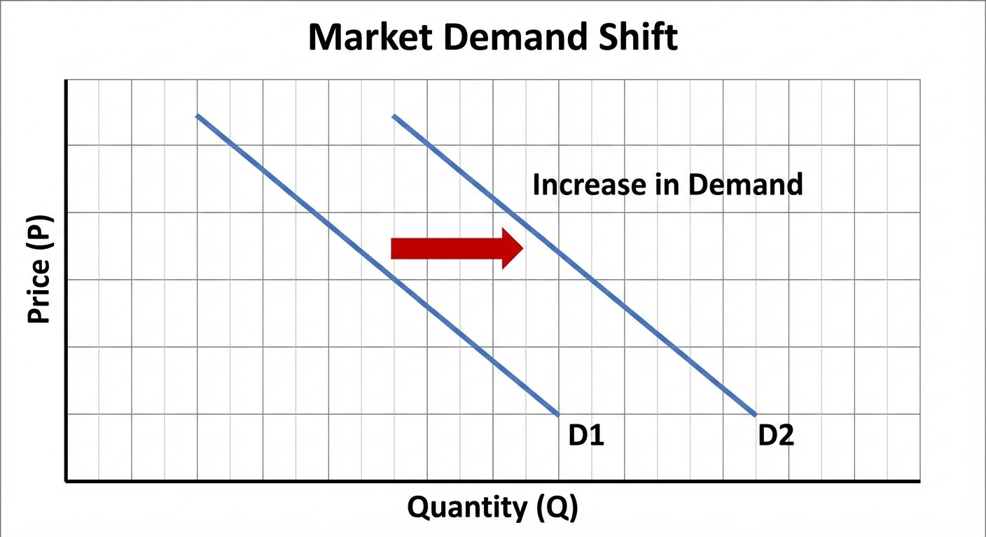
- Change in Quantity Demanded: Caused ONLY by a change in the product's own price. This is a movement along the curve.
- Change in Demand: Caused by non-price factors (shifters). This shifts the entire curve left (decrease) or right (increase).
Shifters of Demand (TRIBE or MERIT)
Use the acronym TRIBE to remember why demand shifts:
- T - Tastes and Preferences: Trends, marketing, scares (e.g., spinach has e-coli).
- R - Related Goods Prices:
- Substitutes: Price of Pepsi $\uparrow$ $\rightarrow$ Demand for Coke $\uparrow$ (Direct relationship).
- Complements: Price of Peanut Butter $\uparrow$ $\rightarrow$ Demand for Jelly $\downarrow$ (Inverse relationship).
- I - Income:
- Normal Goods: Income $\uparrow$ $\rightarrow$ Demand $\uparrow$ (e.g., weakury cars).
- Inferior Goods: Income $\uparrow$ $\rightarrow$ Demand $\downarrow$ (e.g., instant noodles, used cars).
- B - Buyers (Number of Consumers): More population $\rightarrow$ More demand.
- E - Expectations: If you think price will go up next week, you buy NOW (Demand $\uparrow$).
1.5 Supply
The Law of Supply
There is a direct relationship between Price ($P$) and Quantity Supplied ($Q_s$).
- As $P \uparrow$, $Q_s \uparrow$
- As $P \downarrow$, $Q_s \downarrow$
This creates an upward-sloping curve. Producers want to produce more when they can sell for a higher price.
Shifters of Supply (ROTTEN)
Use the acronym ROTTEN to remember why supply shifts:
- R - Resource Costs (Inputs): If labor or raw materials get expensive, Supply $\downarrow$ (shifts left).
- O - Other Goods' Prices: If a farmer can sell corn for way more than wheat, they will switch fields to corn. Supply of wheat $\downarrow$.
- T - Taxes and Subsidies:
- Tax on producers = Supply $\downarrow$.
- Subsidy (government pays producer) = Supply $\uparrow$.
- T - Technology: Better tech always increases efficiency. Supply $\uparrow$.
- E - Expectations: If a producer expects high prices later, they might hold back stock now. Supply $\downarrow$.
- N - Number of Sellers: More firms entering the market = Supply $\uparrow$.

1.6 Market Equilibrium
Equilibrium Price and Quantity
Equilibrium occurs where the Demand curve intersects the Supply curve ($Qd = Qs$). At this price, there is no tendency for the price to change.

Disequilibrium
- Shortage (Excess Demand):
- Price is below equilibrium.
- $Qd > Qs$.
- Market pressure pushes price UP.
- Surplus (Excess Supply):
- Price is above equilibrium.
- $Qs > Qd$.
- Market pressure pushes price DOWN.
Understanding Shifts (Single vs. Double)
Single Shifts
- Demand Increases: Price $\uparrow$, Quantity $\uparrow$
- Demand Decreases: Price $\downarrow$, Quantity $\downarrow$
- Supply Increases: Price $\downarrow$, Quantity $\uparrow$
- Supply Decreases: Price $\uparrow$, Quantity $\downarrow$
Double Shifts (The "Indeterminate" Rule)
When BOTH curves shift simultaneously, one variable (Price or Quantity) will be known, but the other will be indeterminate (ambiguous) without specific numbers.
- Example: Demand Increases AND Supply Increases.
- Demand $\uparrow$ pushes $P \uparrow, Q \uparrow$
- Supply $\uparrow$ pushes $P \downarrow, Q \uparrow$
- Result: $Q$ definitely increases (both push it up). $P$ is indeterminate (one pushes up, one pushes down).
Market Efficiency
- Productive Efficiency: Producing at the lowest possible cost (any point on the Supply curve or PPC).
- Allocative Efficiency: Producing the amount society most desires compared to costs. This occurs at Market Equilibrium ($S=D$), where Marginal Benefit equals Marginal Cost.
Common Mistakes & Pitfalls
- Money is NOT Capital: In AP Macro, "Capital" refers effectively to tools and machinery. Don't say "the company needs more capital" when you mean they need money. Say "financial capital" if you must.
- Change in Demand vs. Qty Demanded:
- "Price went up, so demand went down" is WRONG.
- "Price went up, so quantity demanded went down" is CORRECT.
- Price is NOT a Shifter: Price never shifts the curve. It moves you along the curve. Only things like Income, Tech, or Tastes shift the curve.
- Mixing up Input/Output Math for Comparative Advantage:
- Memorize: Output = Other goes Over.
- Memorize: Input = Other goes Under.
- Double Shift Certainty: If two curves move, you cannot say for sure what happens to both Price and Quantity. One is always indeterminate.