Generating Magnetic Fields: From Current to B-Field
The Biot-Savart Law
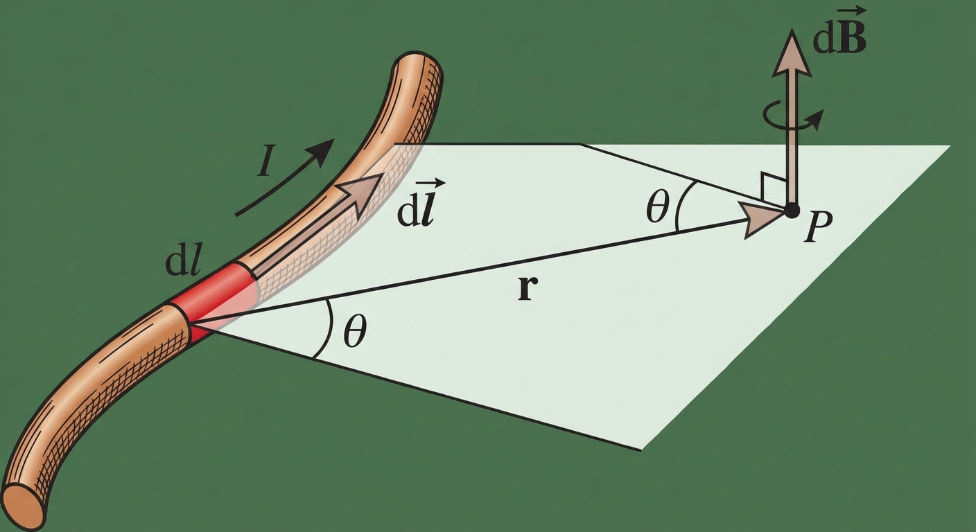
The Biot-Savart Law is the fundamental principle used to calculate the magnetic field produced by a steady electric current. It plays a role in magnetism analogous to Coulomb's Law in electrostatics. While Coulomb's Law calculates the electric field from a point charge, the Biot-Savart Law calculates the differential magnetic field contribution ($d\vec{B}$) from a differential current element ($Id\vec{l}$).
The Formula
For a small segment of wire of length $d\vec{l}$ carrying current $I$, the magnetic field $d\vec{B}$ at a point $P$ is given by:
Where:
- $\mu_0$ is the permeability of free space ($4\pi \times 10^{-7} \ T\cdot m/A$).
- $I$ is the steady current (Amperes).
- $d\vec{l}$ is the vector representing the infinitesimal length element pointing in the direction of current.
- $\hat{r}$ is the unit vector pointing from the current element to the point of observation $P$.
- $r$ is the distance from the current element to point $P$.
Key Principles
- Vector Nature: Since this involves a cross product ($d\vec{l} \times \hat{r}$), the resulting magnetic field is always perpendicular to both the current direction and the position vector. You must use the Right-Hand Rule to determine direction.
- Superposition: To find the total magnetic field $\vec{B}$, you must integrate the contribution over the entire length of the current distribution:
Worked Example: Field of a Finite Straight Wire
Consider a straight wire of length $L$ lying on the x-axis from $-L/2$ to $L/2$. Calcuate the $B$-field at a point $P$ located distance $y$ above the center of the wire.
- Setup: $d\vec{l} = dx \ \hat{i}$. The vector $\vec{r}$ points from $x$ to $y$, so magnitude $r = \sqrt{x^2 + y^2}$.
- Cross Product: The angle $\theta$ between the wire and $\vec{r}$ satisfies $\sin(\theta) = \frac{y}{\sqrt{x^2+y^2}}$. The direction is $\hat{k}$ (out of page).
- Integration:
Using trigonometric substitution (where $x = y \tan \alpha$), the result simplifies to:
Ampere’s Law
While the Biot-Savart Law is universal, the integration can be mathematically difficult. Ampere’s Law relates the integrated magnetic field around a closed loop to the electric current passing through the loop. It is highly effective for calculating magnetic fields in situations with high symmetry (cylindrical or planar).
The Formula
- $\oint \vec{B} \cdot d\vec{l}$: The line integral of the magnetic field around a closed path (Amperian Loop).
- $I_{enc}$: The net current enclosed by (passing through) the area defined by the Amperian Loop.
Applying Ampere’s Law
To use this law effectively, you must choose an Amperian Loop such that:
- The magnetic field $\vec{B}$ is constant in magnitude everywhere on the loop.
- The angle between $\vec{B}$ and $d\vec{l}$ is constant (usually $0^\circ$ or $90^\circ$).
When these conditions are met, the vector dot product simplifies to standard multiplication, allowing you to pull $B$ out of the integral:
| Feature | Biot-Savart Law | Ampere's Law |
|---|---|---|
| Analogy | Coulomb's Law | Gauss's Law |
| Applicability | Any steady current distribution | Highly symmetric currents |
| Math Difficulty | High (Vector calculus integration) | Low (Algebraic if symmetry exists) |
Magnetic Fields of Common Configurations
There are four specific geometries you must master for the AP Physics C exam.
1. The Long Straight Wire
For an infinitely long wire carrying current $I$, we use a circular Amperian loop of radius $r$.
- Circumference: $2\pi r$
- Symmetry: $\vec{B}$ is tangent to the circle everywhere.
- Result:
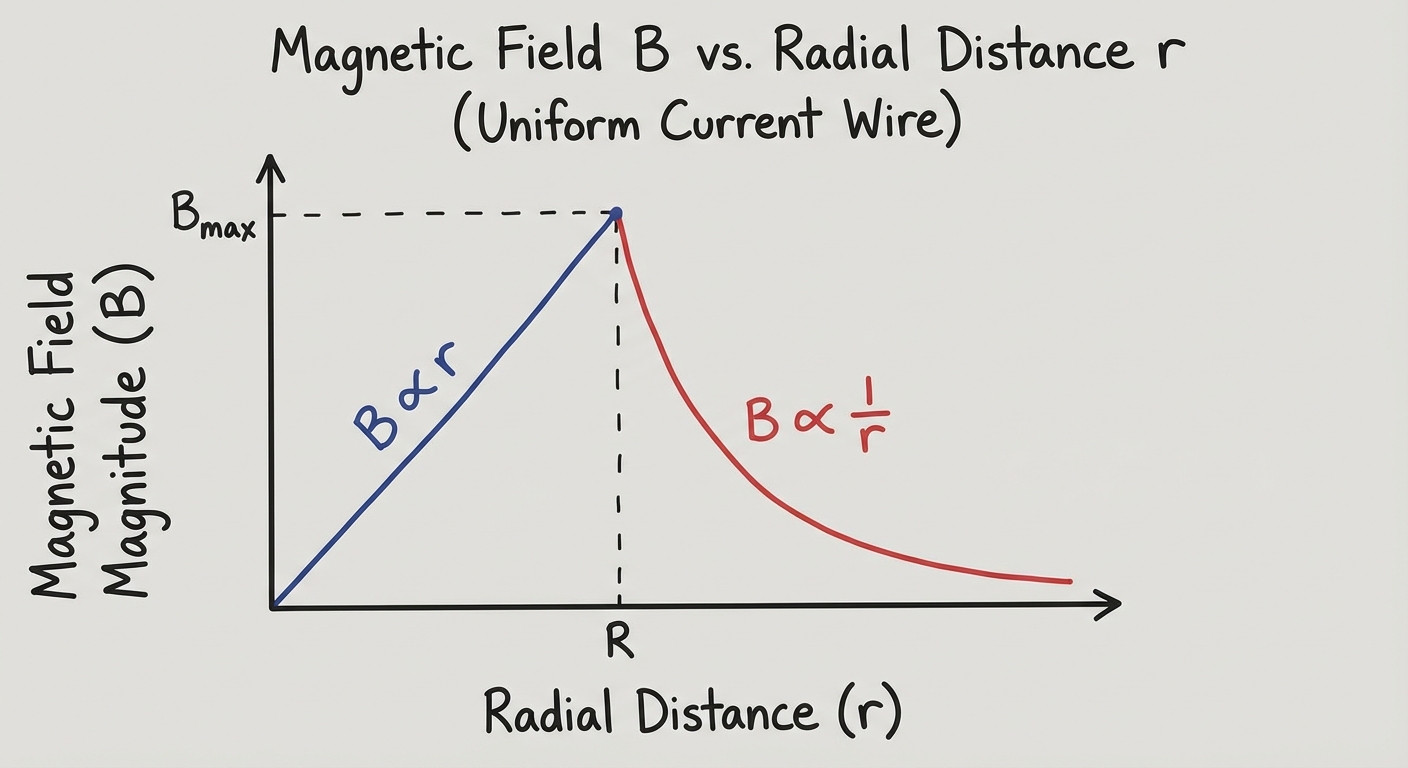
Note: If the wire has a physical radius $R$ and uniform current density $J$, the field inside the wire ($r < R$) increases linearly with $r$, while the field outside ($r > R$) drops off as $1/r$.
2. Force Between Parallel Wires
Two parallel wires carrying currents $I1$ and $I2$ separated by distance $d$ exert magnetic forces on each other.
- Wire 1 creates a field $B1 = \frac{\mu0 I_1}{2\pi d}$ at the location of Wire 2.
- Wire 2 experiences a force $F = I2 L B1$.
- Force per unit length:
Memory Aid:
- Currents in the SAME direction ATTRACT.
- Currents in OPPOSITE directions REPEL.
3. The Solenoid
A solenoid is a long coil of wire consisting of many loops.
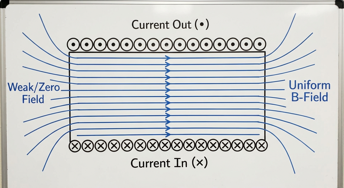
- Ideal Solenoid: Long length compared to diameter. The field inside is uniform; the field outside is approximately zero.
- Derivation: Use a rectangular Amperian loop partially inside and partially outside the solenoid.
- Formula:
- Here, $n = N/L$ is the number of turns per unit length (turns per meter), NOT the total turns $N$.
4. The Toroid
A toroid is essentially a solenoid bent into a circle (like a donut).
- Field Inside: The field is confined entirely inside the coils.
- Formula: Derived using a circular Amperian loop inside the toroid of radius $r$.
- Here, $N$ is the total number of turns.
- Note that $B$ is not uniform; it is stronger at the inner radius and weaker at the outer radius ($1/r$ dependence).
Common Mistakes & Pitfalls
- Confusing $n$ and $N$: In solenoid problems, students often plug in the total turns $N$ instead of the turn density $n$. Remember: $n = N/L$.
- The "Radius" Trap in Biot-Savart: The denominator in Biot-Savart is $r^2$, but the integration often involves variables like $x^2 + y^2$. Don't forget to rewrite $d\vec{l}$ and $r$ in terms of the integration variable properly before integrating.
- Right-Hand Rule Orientation: When using Ampere's Law, the direction of the integration path determines the sign of the enclosed current. If you curl your fingers in the direction of integration, your thumb points in the direction of positive current.
- Enclosed Current: For thick wires or coaxial cables, calculating $I{enc}$ often requires a ratio of areas (current density $J = I{total}/A{total}$) if the loop is inside the conductor. Do not assume $I{enc} = I_{total}$ if $r < R$.