Unit 9: Inference for Quantitative Data: Slopes
Introduction to Inference for Linear Regression
In previous units, you learned how to describe the relationship between two quantitative variables using the Least Squares Regression Line (LSRL). In Unit 9, we move from description to inference. We acknowledge that our sample data is just one of many possible samples we could have drawn from a larger population.
We use the sample regression line to estimate the true population regression line and to determine if there is a statistically significant linear relationship between the variables.
The Regression Models
It is crucial to distinguish between the statistics (calculated from sample data) and parameters (theoretical truth of the population).
| Population Model (Theoretical) | Sample Model (Calculated) | |
|---|---|---|
| Equation | $\mu_y = \alpha + \beta x$ | $\hat{y} = a + bx$ |
| Y-intercept | $\alpha$ (Alpha) | $a$ (statistic) |
| Slope | $\beta$ (Beta) | $b$ (statistic) |
| Residuals | $\epsilon$ (Error) | $y - \hat{y}$ |
- $\beta$ (Population Slope): The true amount the response variable ($y$) changes for every one-unit increase in the explanatory variable ($x$) in the entire population.
- $b$ (Sample Slope): An unbiased estimator of $\beta$.
The Sampling Distribution of the Slope
When verifying conditions are met, the sampling distribution of the sample slope ($b$) follows a specific pattern. If we took many random samples of the same size $n$ from the population and calculated the slope for each, the distribution of those slopes would be centered at the true slope $\beta$.
Properties of the Sampling Distribution
- Shape: Approximately Normal (if conditions are met).
- Center: $\mu_b = \beta$ (The mean of the sample slopes is the true population slope).
- Spread: The standard deviation of the slope, $\sigma_b$, describes how much the sample slope varies from sample to sample.
Standard Error of the Slope ($SE_b$)
Because we rarely know the true population standard deviation ($
\sigma$), we use the Standard Error estimated from the sample data.
The Standard Error of the slope is given by:
Where:
- $s$ = Standard deviation of the residuals (spread of $y$ about the line).
- $s_x$ = Standard deviation of the explanatory variable ($x$).
- $n$ = Sample size.
Note: On the AP exam, $SE_b$ is almost always provided in a computer output table. You rarely need to calculate it by hand from raw data.
The standardized test statistic follows a $t$-distribution with degrees of freedom:
Conditions for Inference (LINER)
To construct a confidence interval or perform a hypothesis test for the slope, the LINER conditions must be checked.
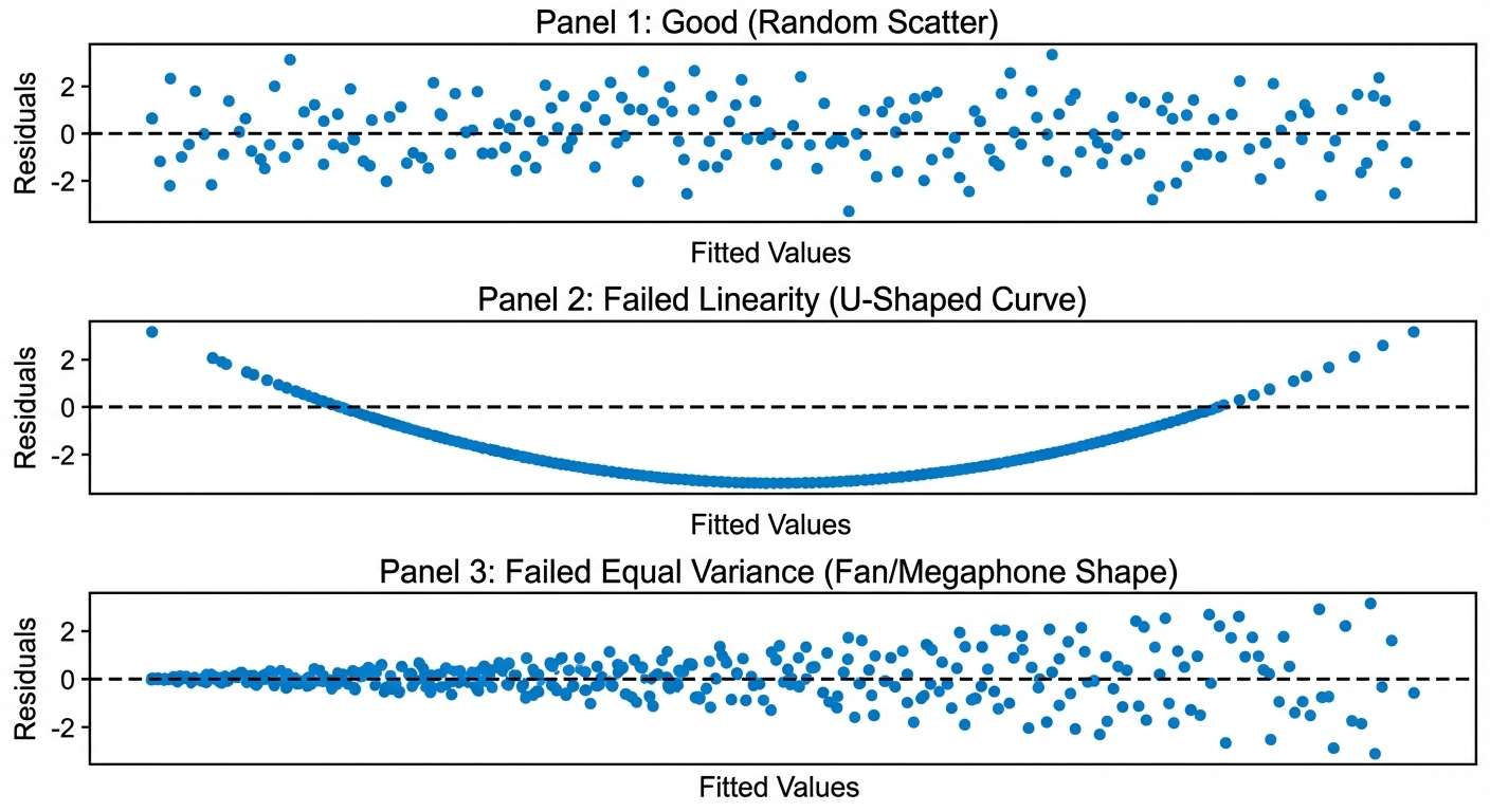
1. Linear
Concept: The true relationship between $x$ and $y$ must be linear.
- Check: Look at the scatterplot of $x$ vs. $y$ (should look straight, not curved).
- Check: Look at the Residual Plot. There should be no leftover curved pattern. A U-shape in the residual plot indicates a non-linear relationship.
2. Independent
Concept: Individual observations must be independent.
- Check: If sampling without replacement, the population size $N$ must be at least 10 times the sample size $n$ ($10\%$ condition).
3. Normal
Concept: The response variable $y$ varies normally around the true regression line.
- Check: Look at a histogram or Normal Probability Plot of the residuals. It should show no strong skewness or outliers.
4. Equal Variance (Homoscedasticity)
Concept: The standard deviation of $y$ () is the same for all values of $x$.
- Check: Look at the Residual Plot. The vertical spread of residuals should be roughly consistent across all $x$-values.
- Bad Sign: A "fan shape" (residuals getting much wider or narrower as $x$ increases) violates this condition.
5. Random
Concept: Data comes from a random sample or randomized experiment.
- Check: Look for "randomly selected" or "random assignment" in the problem description.
Interpreting Computer Output
AP Statistics questions frequently provide regression analysis generated by software (like Minitab, JMP, or Excel). You must know how to locate the relevant statistics.
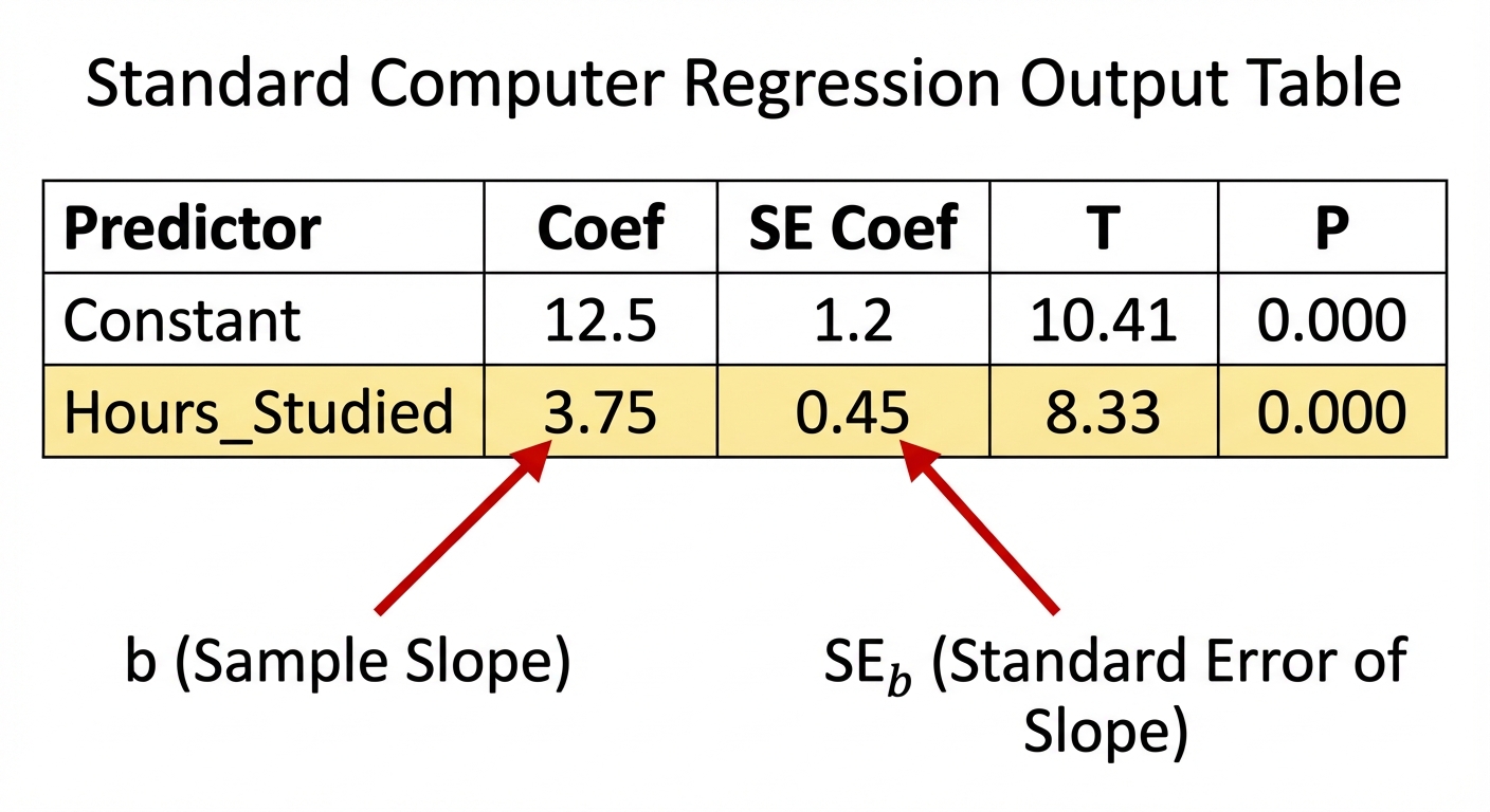
Key Components of the Output Table:
| Term / Variable | Coef (Coefficient) | SE Coef (Standard Error) | T-Value (T-stat) | P-Value |
|---|---|---|---|---|
| Constant (Intercept) | $a$ (y-intercept) | $SE_a$ | $t$ for intercept | $p$ for intercept |
| Variable Name (Slope) | $b$ (Slope) | $SE_b$ (SE of Slope) | $t$ for slope | $p$ for slope |
- Coef (Slope): This is $b$. Used for the regression equation $\hat{y} = a + bx$.
- SE Coef: This is standard error ($SEb$). Used in the denominator of the t-statistic formula or margin of error ($t^* \times SEb$).
- S: The standard deviation of the residuals.
- r-sq: The coefficient of determination ($r^2$).
Confidence Interval for the Slope
A confidence interval estimates the true population slope $\beta$.
Formula
- $b$: Sample slope.
- $t^*$: Critical value for $df = n-2$ and confidence level $C\%$.
- $SE_b$: Standard error of the slope.
Worked Example: SAT Scores
Scenario: A researcher wants to see if SAT Verbal scores predict SAT Math scores. A random sample of 15 students is selected. A regression analysis yields:
- Equation: $\widehat{Math} = 209.55 + 0.675(Verbal)$
- SE of Slope ($SE_b$) = 0.056
- $n = 15$
Task: Construct and interpret a 95% confidence interval for the true slope.
1. State: We will estimate the slope $\beta$ of the true regression line relating SAT Verbal scores to SAT Math scores at a 95% confidence level.
2. Plan: Identify the procedure: One-sample t-interval for slope.
- Assumption Check: Assume LINER conditions are met based on the problem statement.
3. Do:
- $b = 0.675$
- $SE_b = 0.056$
- $df = 15 - 2 = 13$
- Find $t^$ for 95% confidence and $df=13$ using inverse-t: $t^ \approx 2.160$
4. Conclude:
We are 95% confident that the interval from 0.554 to 0.796 captures the slope of the true regression line relating SAT Verbal scores to SAT Math scores.
Interpretation: For every 1-point increase in SAT Verbal score, we are 95% confident the average increase in SAT Math score is between 0.554 and 0.796 points.
Hypothesis Test for the Slope
Most often, we test if there is any linear relationship. If $\beta = 0$, the regression line is horizontal, meaning $x$ has no predictive power for $y$ (no linear relationship).
Hypotheses
- Null Hypothesis ($H_0$): $\beta = 0$ (There is no linear relationship between $x$ and $y$).
- Alternative Hypothesis ($H_a$):
- $\beta \neq 0$ (There is a linear relationship).
- $\beta > 0$ (There is a positive linear relationship).
- $\beta < 0$ (There is a negative linear relationship).
Test Statistic Formula
Usually $\beta0 = 0$, so:
Worked Example: Tennis Serves
Scenario: Data from 10 randomly selected tennis players compares 'Old Racket Speed' ($x$) vs 'New Racket Speed' ($y$).
- Computer Output: Slope ($b$) = 1.05, $SE_b$ = 0.12.
- Question: Is there convincing evidence of a positive linear relationship?
1. State:
- $H_0: \beta = 0$
- $H_a: \beta > 0$
- Where $\beta$ is the true slope relating Old Racket Speed to New Racket Speed.
- $
\alpha = 0.05$
2. Plan:
- t-test for slope.
- Check Conditions: Random sample (given), Scatterplot linear (assume), Residuals normal (assume), Equal variance (assume).
3. Do:
- $t = \frac{1.05 - 0}{0.12} = 8.75$
- $df = 10 - 2 = 8$
- $P\text{-value} = P(t > 8.75)$ using $tcdf(8.75, 9999, 8) \approx 0.000006$
4. Conclude:
Because the p-value ($0.000006$) is less than $\alpha$ ($0.05$), we reject $H_0$. There is convincing evidence that there is a positive linear relationship between old racket speeds and new racket speeds.
Common Mistakes & Pitfalls
Confusing $b$ and $\beta$:
- $b$ is the sample slope (the number you calculated).
- $\beta$ is the population slope (the number you are trying to estimate).
- Correction: Hypotheses always use Greek letters ($H0: \beta = 0$, NEVER $H0: b = 0$).
Misinterpreting the Interval:
- Mistake: "We are 95% confident the sample slope falls in this interval." (We already know the sample slope).
- Mistake: "95% of the data points fall in this interval." (No, this is about the slope of the line, not the individual data points).
- Correction: Always refer to the "slope of the true regression line."
Forgetting Degrees of Freedom:
- Mistake: Using $n-1$ like in one-variable inference.
- Correction: For linear regression slope, $df = n - 2$ (because we estimated two parameters, $\alpha$ and $\beta$, to fit the line).
Reading the Wrong Line in Computer Output:
- Mistake: Using the "Constant" row for inference.
- Correction: Always look for the row with the variable name to find slope statistics.
Checking Normality of Raw Data:
- Mistake: Checking if $x$ or $y$ distributions are Normal.
- Correction: You must check if the residuals are Normal. $x$ and $y$ do not need to be symmetric distributions themselves, but the errors around the line must be.