AP Macroeconomics Unit 3: National Income and Price Determination Study Guide
Equilibrium in the AD-AS Model
Macroeconomic equilibrium occurs when the aggregate quantity of output demanded equals the aggregate quantity of output supplied. In the AD-AS model, this is visualized as the intersection of your demand and supply curves. Understanding how to locate and manipulate this equilibrium is the foundation of analyzing economic shocks.
Short-Run Equilibrium
Short-Run Equilibrium exists when the aggregate quantity of goods and services demanded equals the aggregate quantity of goods and services supplied at a specific price level. Graphically, this is the intersection of the Aggregate Demand (AD) curve and the Short-Run Aggregate Supply (SRAS) curve.
- Equilibrium Price Level ($PL_e$): The price level where the AD and SRAS curves intersect.
- Equilibrium Real GDP ($Y_e$): The level of output produced at that intersection.
If the price level is above equilibrium, there is a surplus of goods/services, putting downward pressure on prices. If the price level is below equilibrium, there is a shortage, putting upward pressure on prices.

Output Gaps
Ideally, short-run equilibrium occurs exactly at the Full-Employment level of output ($Y_f$), represented by the vertical Long-Run Aggregate Supply (LRAS) curve. However, the economy frequently fluctuates, leading to gaps.
Recessionary Gap ($Ye < Yf$):
- Current real GDP is less than potential GDP.
- Unemployment is higher than the Natural Rate of Unemployment (NRU).
- Graphically: The intersection of AD and SRAS is to the left of the LRAS curve.
Inflationary Gap ($Ye > Yf$):
- Current real GDP is greater than potential GDP.
- Unemployment is lower than the NRU (economy is overheating).
- Graphically: The intersection of AD and SRAS is to the right of the LRAS curve.
Stagflation:
- Caused by a negative supply shock (SRAS shifts left).
- Results in higher price levels (inflation) AND lower output (stagnation/recession).
- This is the worst-case scenario because traditional demand-side policies treat one problem while worsening the other.

Short-Run and Long-Run Equilibrium
While short-run equilibrium is determined by current AD and SRAS, the economy naturally moves toward long-run equilibrium over time without government intervention. This process rests on the flexibility of wages and resource prices.
The Self-Correction Mechanism
Classical economic theory suggests that the economy will self-correct in the long run resulting in a return to full employment ($Y_f$).
Scenario 1: Closing a Recessionary Gap (No Intervention)
- situation: High unemployment creates a surplus of labor.
- Adjustment: Nominal wages eventually fall because workers produce less or accept lower pay to get hired.
- Result: Lower input costs allow firms to increase production. SRAS shifts RIGHT.
- Outcome: Price level decreases, Output returns to $Y_f$.
Scenario 2: Closing an Inflationary Gap (No Intervention)
- Situation: Low unemployment creates a shortage of labor.
- Adjustment: Nominal wages eventually rise as workers demand higher pay due to inflation and scarcity.
- Result: Higher input costs force firms to cut production. SRAS shifts LEFT.
- Outcome: Price level increases, Output returns to $Y_f$.
Key Concept: In the long run, we assume wages and prices are flexible. In the short run, they are sticky.
Fiscal Policy
Fiscal Policy refers to the use of government spending ($G$) and taxation ($T$) to influence the economy. These policies are discretionary, meaning they require new laws or actions by Congress/Parliament.
Tools of Fiscal Policy
Since $G$ is a direct component of Aggregate Demand ($AD = C + I + G + X_n$) and Taxes affect Consumption ($C$) and Investment ($I$), Fiscal Policy primarily shifts the AD curve.
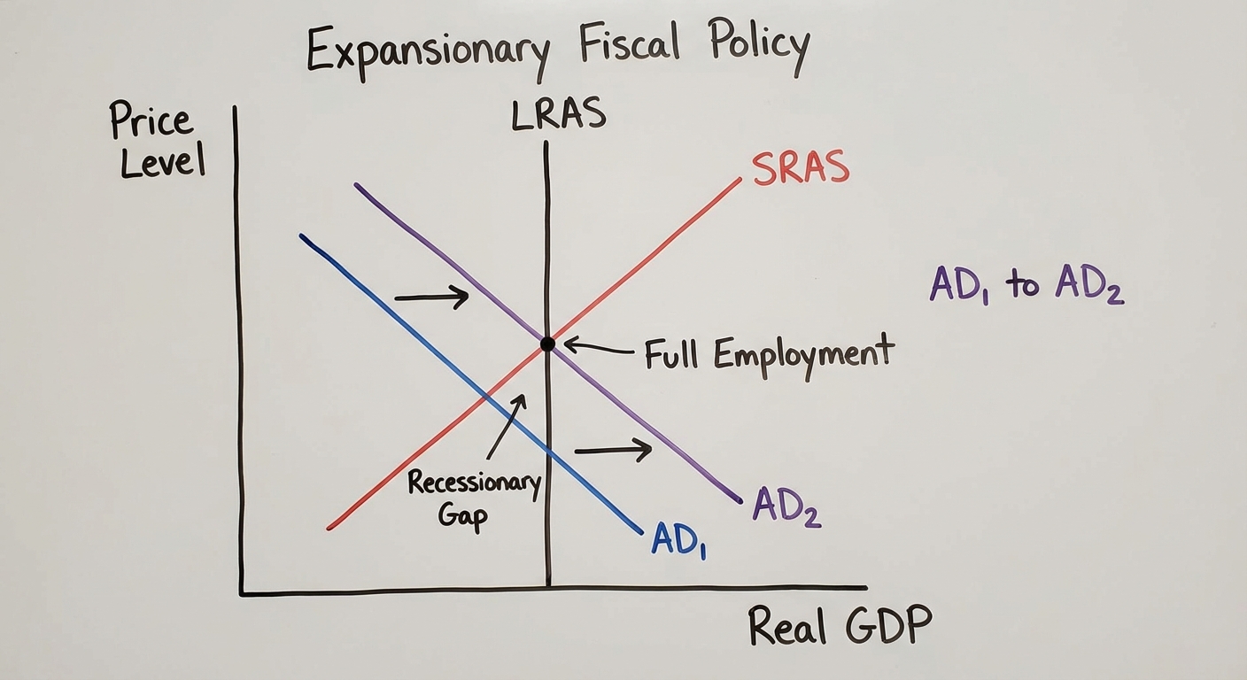
1. Expansionary Fiscal Policy
Used to combat Recession (close a recessionary gap).
- Actions: Increase Government Spending ($ o ext{direct } riangle AD$) OR Decrease Taxes ($ o riangle ext{Disposable Income} o riangle C$).
- Goal: Shift AD to the Right.
- Side Effect: Can lead to a budget deficit and potentially higher price levels (inflation).
2. Contractionary Fiscal Policy
Used to combat Inflation (close an inflationary gap).
- Actions: Decrease Government Spending OR Increase Taxes.
- Goal: Shift AD to the Left.
- Side Effect: Can lead to a budget surplus (or reduced deficit) but lowers Real GDP.
Comparison Table
| Economic Problem | Policy Type | Spending ($G$) | Taxes ($T$) | Target Shift | Impact on PL | Impact on Output |
|---|---|---|---|---|---|---|
| Recession | Expansionary | Increase | Decrease | AD $ | ||
| ightarrow$ Right | Increases | Increases | ||||
| Inflation | Contractionary | Decrease | Increase | AD $ | ||
| ightarrow$ Left | Decreases | Decreases |
The Multiplier Effect
Fiscal policy is powerful because of the multiplier effect. An initial change in spending ripples through the economy, creating a larger change in total Real GDP.
Where $MPC$ = Marginal Propensity to Consume and $MPS$ = Marginal Propensity to Save.
Note: The Spending Multiplier is always mathematically larger (in absolute value) than the Tax Multiplier. Therefore, a change in Government Spending has a greater impact on GDP than an equal change in taxes.
Automatic Stabilizers
Not all fiscal policy requires a new vote in Congress. Automatic Stabilizers are mechanisms built into the economy that naturally counter fluctuations in the business cycle without specific new government action.
How They Work
Stabilizers work by changing Disposable Income automatically as GDP fluctuates.
Progressive Income Information Taxes:
- Scenario (Inflation): When incomes rise, individuals move into higher tax brackets. This increases the average tax rate, slowing down the growth of Disposable Income and Consumption, which dampens AD.
- Scenario (Recession): When incomes fall, tax liabilities drop significantly, preserving some Disposable Income and preventing AD from crashing too hard.
Transfer Payments (Unemployment Insurance/Welfare):
- Scenario (Recession): More people apply for unemployment benefits. Government spending (transfers) automatically increases, sustaining consumption levels.
- Scenario (Expansion): Fewer people need benefits. Government spending automatically decreases, preventing the economy from overheating.
Mnemonic: Stabilizers act like the shock absorbers on a car. They don't drive the car (shift the trend), but they smooth out the bumps (fluctuations in the business cycle).
Common Mistakes & Pitfalls
Confusing Fiscal Actions with Monetary Policy:
- Mistake: Thinking the Federal Reserve/Central Bank enacts fiscal policy.
- Correction: Fiscal Policy = Congress/Government (Taxes & Spending). Monetary Policy = Central Bank (Money Supply & Interest Rates).
Shifting the Wrong Curve:
- Mistake: Moving the AS curve when the government changes taxes.
- Correction: In this unit, Fiscal Policy (T and G) shifts Aggregate Demand (AD). Taxes affect consumers ($C$) and businesses ($I$), which are components of AD.
Self-Correction Logic:
- Mistake: Thinking the government must act to fix a gap.
- Correction: The economy generally self-corrects in the long run via SRAS shifts (wage adjustments). Government policy is used to speed up the process by shifting AD.
Automatic vs. Discretionary:
- Mistake: Calling a new tax cut law an "automatic stabilizer."
- Correction: If politicians have to vote on it, it operates as Discretionary policy. Automatic stabilizers happen by default based on existing laws (e.g., you earn less, you automatically pay less tax).