Comprehensive Guide to Chi-Square Inference
Chi-Square Tests Analysis and Applications
In AP Statistics, Unit 8 focuses on analyzing categorical data. While proportions ($z$-tests) handle binary categorical data (success/failure), Chi-Square ($ \chi^2$) tests allow us to analyze variables with multiple categories. These tests measure how far our observed data deviates from what we would expect to see if a specific null hypothesis were true.
The Chi-Square Statistic Basic Concepts
Before diving into specific tests, it is crucial to understand the underlying statistic used for all three tests in this unit. The Chi-Square statistic measures the discrepancy between observed counts and expected counts.
General Formula
The formula for the Chi-Square statistic is:
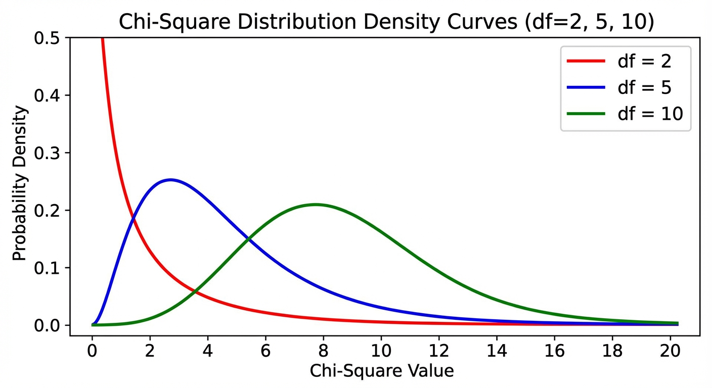
Key Properties of the Chi-Square Distribution
- Right-Skewed: Unlike the Normal distribution, the $\chi^2$ curve is skewed to the right. As degrees of freedom increase, it becomes more symmetric (normal-like).
- Positive Values Only: Since the numerator is squared, $\chi^2 \ge 0$. A value of 0 means Observed perfectly matches Expected.
- Area in the Tail: These tests are always "one-sided" in practice because any significant deviation (positive or negative) increases the $\chi^2$ value. We look for the area in the right tail greater than our calculated statistic.
Chi-Square Goodness of Fit Test
The Goodness of Fit test determines if a sample distribution of a single categorical variable matches a claimed population distribution.
Conditions
- Random: The data must come from a random sample or randomized experiment.
- 10% Condition: If sampling without replacement, $n < 10\%$ of the population.
- Large Counts: All expected counts must be at least 5. (Note: Do not check observed counts for this condition).
Hypotheses
- $H0$: The distribution of [variable] is the same as the claimed distribution (or specifies proportion $p1=.., p_2=…$).
- $H_a$: The distribution of [variable] is not the same as the claimed distribution.
Degrees of Freedom (df)
Example Scenario: The Die Roll
Scenario: A gamer suspects a 6-sided die is weighted. They roll it 60 times.
Expected Counts: If fair, $P(1)=P(2)…=1/6$. Expected count for each face = $60 \times (1/6) = 10$.
Observed: 1: 5, 2: 8, 3: 9, 4: 8, 5: 10, 6: 20.
Calculation:
If the P-value associated with this $\chi^2$ (at $df = 5$) is below $\alpha$ (0.05), we reject $H_0$ and conclude the die is not fair.
Chi-Square Test for Homogeneity
The Test for Homogeneity compares the distribution of a categorical variable across two or more distinct populations or treatments.
Distinctive Feature
This test involves multiple samples (e.g., a sample of Freshmen, a sample of Sophomores) or random assignment to multiple treatment groups.
Hypotheses
- $H_0$: The distribution of [variable] is the same for [Population 1] and [Population 2].
- $H_a$: The distribution of [variable] is different for [Population 1] and [Population 2].
Calculating Expected Counts (Two-Way Tables)
When data is in a matrix (Two-Way Table), the expected count for any cell is:
Degrees of Freedom
Use Case
Do Freshmen, Juniors, and Seniors have the same preference distribution for Prom themes? (3 groups, 1 variable: Theme Preference).
Chi-Square Test for Independence
The Test for Independence determines if there is an association between two categorical variables within a single population.
Distinctive Feature
This test involves one single sample, cross-classified by two variables.
Hypotheses
- $H_0$: There is no association between [Variable A] and [Variable B] (they are independent).
- $H_a$: There is an association between [Variable A] and [Variable B] (they are dependent).
Math & Calculations
The math for Independence is identical to Homogeneity:
- Expected counts use the Row/Column total formula.
- $\chi^2$ statistic is calculated the same way.
- Degrees of freedom are $(r-1)(c-1)$.
Use Case
Take one sample of 500 adults. Record their Gender and their Favorite Movie Genre. Are Gender and Genre associated?
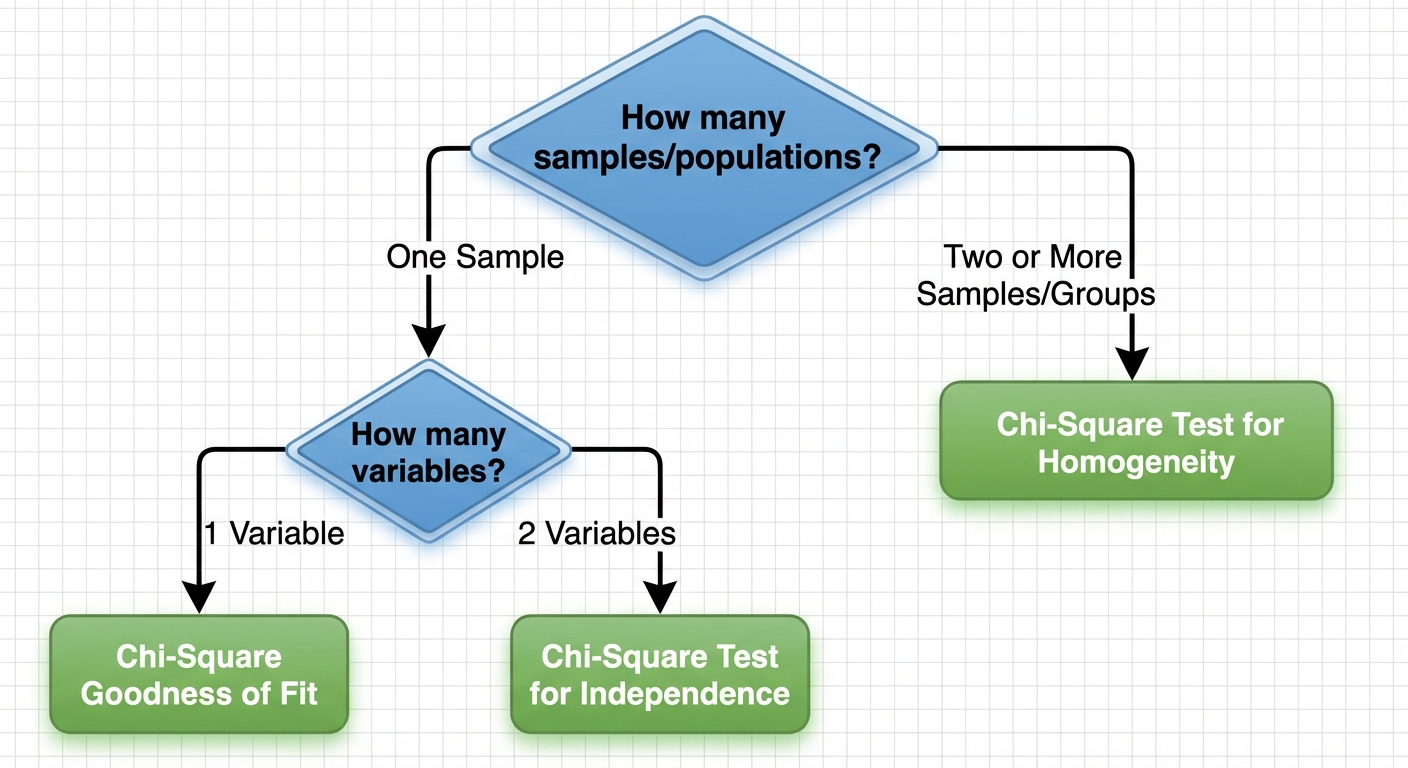
Selecting an Appropriate Inference Procedure
Students often confuse Homogeneity and Independence because the math is identical. The difference lies entirely in the study design (how the data was collected).
The Decision Matrix
| Feature | Goodness of Fit | Homogeneity | Independence |
|---|---|---|---|
| Number of Samples | One Sample | Two or more samples (or groups) | One Sample |
| Variables | 1 Variable | 1 Variable (compared across groups) | 2 Variables (cross-categorized) |
| Question asked | "Does it match the model?" | "Are the groups the same?" | "Are variables related?" |
Quick Check Routine
- Look at the total 'N': Did we survey 100 people total (Independence), or did we take 100 men and 100 women (Homogeneity)?
- Look at the Hypotheses: Are we comparing distributions (Homogeneity) or looking for a relationship/association (Independence)?
Common Mistakes & Pitfalls
1. Large Counts Condition Error
Mistake: Checking if the Observed counts are $\ge 5$.
Correction: The condition applies to Expected counts. The theoretical model must be robust enough, regardless of what we actually observed.
2. Proportion vs. Counts
Mistake: Entering percentages or proportions into the matrix for calculation.
Correction: Chi-Square tests run on counts (integers) only. You cannot calculate $\chi^2$ from percentages.
3. Phrasing Hypotheses
Mistake: Writing hypotheses for Independence/Homogeneity using symbols (like $\mu$ or $p$).
Correction: These hypotheses are usually written in words.
- Correct: $H_0$: Gender and Political Party are independent.
- Incorrect: $H0: p1 = p_2$ (This is for a z-test, or relies on 2x2 tables only).
4. "Accepting" the Null
Mistake: Concluding that "The distributions are the same" when $P > \alpha$.
Correction: We never prove the null. Modeling phrasing: "We do not have sufficient evidence to conclude the distributions are different."
5. Follow-up Analysis
Recall: If the test is significant (reject $H_0$), look at the individual contributions to the $\chi^2$ sum. The cell with the largest contribution (Observed - Expected deviation) is the main driver of the association or difference.