Unit 2 Guide: Energy and Scalar Fields in Electrostatics
Electric Potential Energy ($U_E$)
Definitions and Concepts
In mechanics, you learned that an object in a gravitational field has gravitational potential energy ($Ug$). Similarly, a system of electric charges possesses Electric Potential Energy ($UE$). This energy arises from the configuration of charges in a system.
- Nature: $U_E$ is a scalar quantity. It has magnitude and algebraic sign ($+$ or $-$), but no direction.
- The System Interpretation: Potential energy belongs to the system of at least two charges, not a single isolated charge.
- Signs:
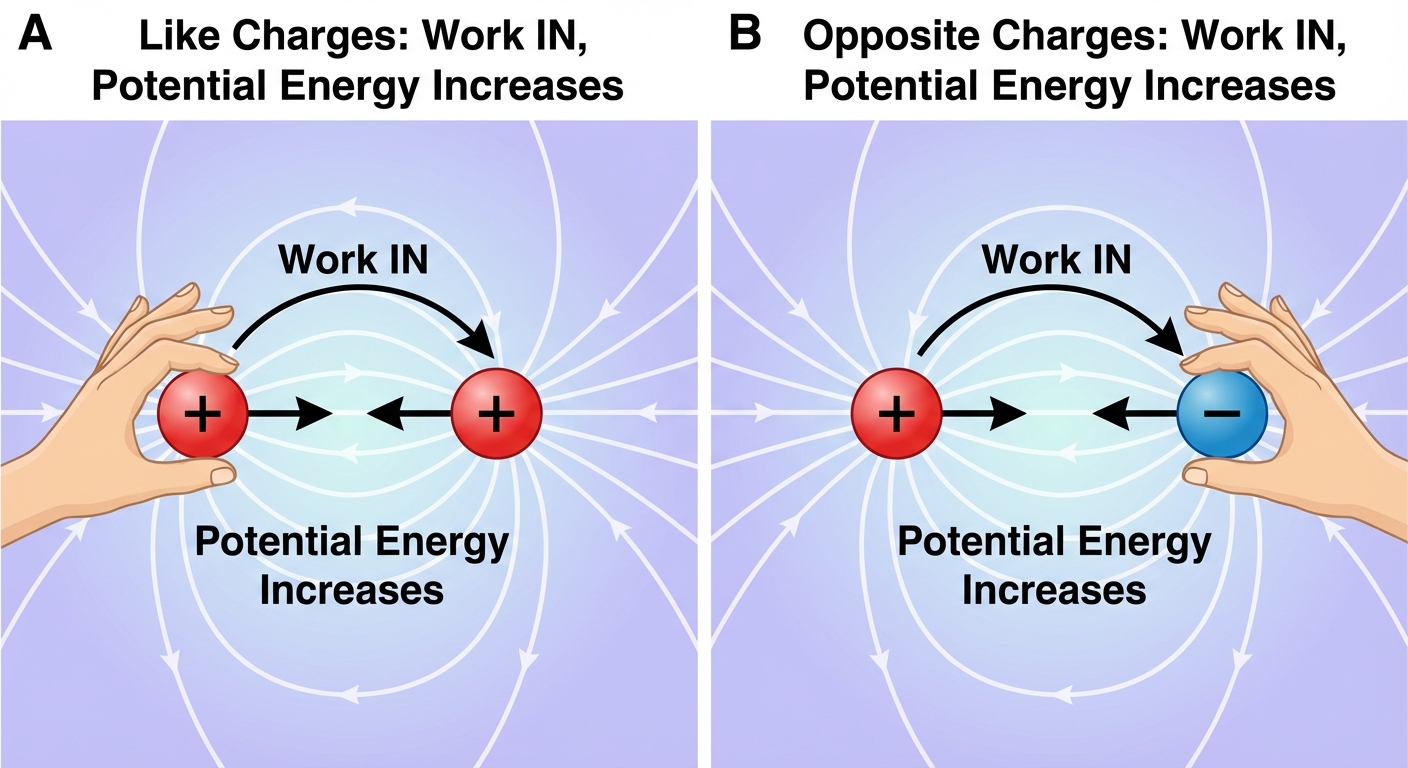
- Positive (+) $U_E$: Represents repulsive interaction (like charges). You must do work to push them together.
- Negative (-) $U_E$: Represents attractive interaction (opposite charges). You must do work to pull them apart.
Formulas and Notation
The electric potential energy stored in a system of two point charges $q1$ and $q2$ separated by a distance $r$ is:
Where:
- $k$: Coulomb’s constant ($8.99 \times 10^9 \text{ N} \cdot \text{m}^2/\text{C}^2$)
- $r$: The distance between the centers of the charges (in meters)
Note: Unlike the electric force formula (Coulomb's Law), the distance is $r$, not $r^2$. Also, you must substitute the signs of the charges into this equation.
Work and Energy
The relationship between Work ($W$) and Electric Potential Energy is governed by the Work-Energy Theorem.
Work done by the Electric Field ($WE$): When the electric force moves a charge directly, the field does positive work, and potential energy decreases.
Work done by an External Force ($W{ext}$): The work required to move a charge against the electric field at constant velocity.
Electric Potential ($V$)
Definitions and Concepts
Start by distinguishing between Potential Energy and Potential.
Electric Potential ($V$) is the electric potential energy per unit charge at a specific location in space. It is a property of the source charges creating the field, independent of any test charge placed there.
- Analogy: If Electric Field ($E$) is like the "force field" per unit charge, Electric Potential ($V$) is like the "energy landscape" or "elevation" per unit charge.
- Unit: The Volt (V), which is equivalent to a Joule per Coulomb ($J/C$).
Formulas
1. Definition based on Energy:
2. Potential due to a single Point Charge:
3. Potential due to Multiple Point Charges (Superposition):
Since potential is a scalar, you simply add the potentials from individual charges algebraically (keeping signs).
Electric Potential Difference (Voltage)
In circuits and labs, we rarely measure absolute potential. We measure Potential Difference ($\%Delta V$) between two points ($A$ and $B$).
This leads to the crucial conservation of energy equation for moving a particle, $q$, through a potential difference:
Relationship Between Field and Potential
The Uniform Field
For algebra-based physics, a very common scenario is a Uniform Electric Field (like between the parallel plates of a capacitor). The relationship between the magnitude of the potential difference and the field strength is:
- $E$: Magnitude of Uniform Electric Field ($V/m$ or $N/C$)
- $d$: Distance parallel to the field lines
Directionality Rules
Understanding the signs is critical without calculus. Use these rules:
- Electric Field vectors point from High Potential to Low Potential.
- Positive charges naturally accelerate toward lower potential (think of a ball rolling down a hill).
- Negative charges naturally accelerate toward higher potential (think of a bubble floating up).
| Concept | Vector vs. Scalar | Point Charge Calc | Dependence on distance |
|---|---|---|---|
| Electric Force ($F_E$) | Vector (Direction matters) | $k \frac{ | q1 q2 |
| Electric Field ($E$) | Vector (Direction matters) | $k \frac{ | Q |
| Potential Energy ($U_E$) | Scalar (Sign matters) | $k \frac{q1 q2}{r}$ | $1/r$ |
| Electric Potential ($V$) | Scalar (Sign matters) | $k \frac{Q}{r}$ | $1/r$ |
Equipotential Lines and Surfaces
Definitions and Concepts
Equipotential Lines (or Isolines) connect points in space that have the same Electric Potential ($V$).
Think of these as topographic contour lines on a map. If you walk along a contour line, your elevation (potential) doesn't change, so gravity does no work. Similarly, if a charge moves along an equipotential line, the electric force does zero work.
Key Rules for Analysis
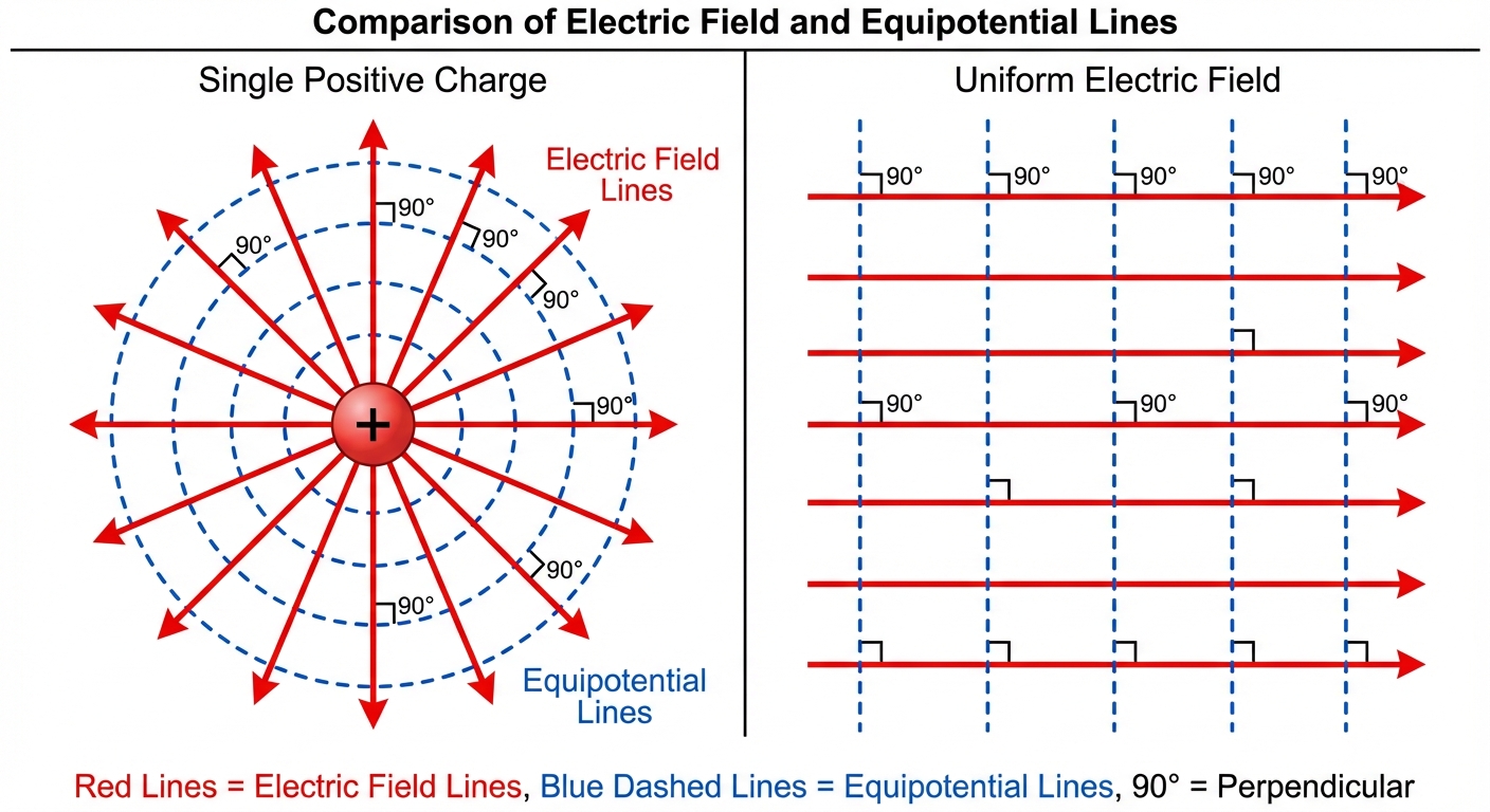
- Perpendicularity: Equipotential lines are always perpendicular to Electric Field lines.
- Field Strength: Closely spaced equipotential lines indicate a strong Electric Field (steep slope). Widely spaced lines indicate a weak field.
- Conductors: The surface (and interior) of a conductor in electrostatic equilibrium is an equipotential surface. The electric field tells us the force, but the fact that charges are not moving (equilibrium) implies no potential difference exists across the conductor.
Common Configurations
- Single Point Charge: Concentric circles. Spacing increases as you move away ($V \propto 1/r$).
- Uniform Field: Parallel lines equally spaced perpendicular to the field vectors.
- Dipole (Positive + Negative): Lines wrap around charges but are squashed between them, with a $V=0$ line right down the middle.
Worked Example: The Three Point Charges
Problem:
Two charges, $+Q$ and $-Q$, are placed on the x-axis at $x = -d$ and $x = +d$, respectively. Determine the Electric Potential ($V$) at the origin ($x=0$). Then, determine the Electric Potential at a point on the y-axis ($y=d$).
Solution:
Step 1: Potential at the Origin
At the origin ($O$), sum the potentials from both charges. Note that $r$ is always positive.
The potential at the center of a dipole is zero.
Step 2: Potential at point P ($0, d$)
First, find the distance $r$ from each charge to point P. Using Pythagoras:
Sum the potentials:
Analysis: For a dipole with equal and opposite charges, the entire bisecting axis (equatorial line) is an equipotential line where $V=0$.
Common Mistakes & Pitfalls
Confusing Vectors and Scalars:
- The Mistake: Breaking Electric Potential calculations into x- and y-components or using trig functions to adding them.
- Correction: $V$ is a scalar. Just add the numbers. If you have a $+2V$ and a $-2V$, the total is $0$, regardless of where the charges are located.
The $r$ vs $r^2$ Trailing:
- The Mistake: Using $1/r^2$ for Potential or Energy calculations.
- Correction: Remember basic calculus logic (even without doing calculus): Energy/Potential is the integral of Force/Field. Integrating power $-2$ gives power $-1$. Potential uses $1/r$.
Dropping the Signs:
- The Mistake: Using absolute values for charges in Potential formulas.
- Correction: For $FE$ and $E$ (vectors), you use magnitudes and determine direction logically. For $UE$ and $V$ (scalars), you must plug in the negative sign for negative charges.
Work and Signs:
- The Mistake: Getting the sign of Work wrong.
- Correction: Remember: If a system does what it "wants" to do naturally (e.g., opposite charges snapping together), Potential Energy decreases ($\%Delta U$ is negative). External work is required to force the system to do the opposite of what it wants.