Unit 5 Guide: The Foundations of Statistical Inference
Sampling Distributions for Proportions and Means
Welcome to Sampling Distributions, arguably the most critical specific topic in AP Statistics. This unit acts as the bridge between descriptive statistics (Units 1–2) and probability (Unit 4) to prepare you for statistical inference (Units 6–9).
When we ask, "How weird is this result assuming the status quo is true?" we are relying entirely on the concepts in this note.
Foundational Concepts: Parameter vs. Statistic
Before diving into the math, you must memorize the distinction between the population and the sample.
- Parameter: A number that describes some characteristic of the population. In practice, the value of a parameter is usually unknown.
- Symbols: $\mu$ (population mean), $p$ (population proportion), $\sigma$ (population standard deviation).
- Statistic: A number that describes some characteristic of a sample. The value of a statistic can be computed directly from the sample data. We use statistics to estimate parameters.
- Symbols: $\bar{x}$ (sample mean), $\hat{p}$ (sample proportion), $s$ (sample standard deviation).
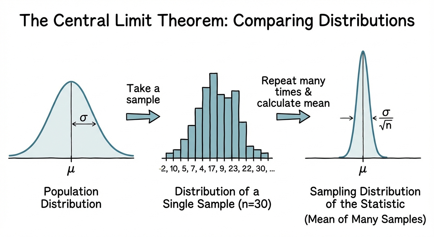
What is a Sampling Distribution?
If you take one sample and calculate the mean, you get one number. If you take a different sample of the same size from the same population, you will likely get a different mean.
Definition: The sampling distribution of a statistic is the distribution of values taken by the statistic in all possible samples of the same size from the same population.
- Biased Estimator: A statistic is biased if the mean of its sampling distribution is not equal to the true value of the parameter being estimated.
- Unbiased Estimator: A statistic is unbiased if the mean of its sampling distribution is equal to the true value of the parameter. (Both $\bar{x}$ and $\hat{p}$ are unbiased estimators).
Sampling Distribution of a Sample Proportion
When dealing with categorical data (Success/Failure, Yes/No), we look at the sample proportion, denoted as $\hat{p}$ (read as "p-hat").
General Properties
If we take repeated samples of size $n$, the distribution of $\hat{p}$ has specific characteristics governing its center, spread, and shape.
1. Center (The Mean)
Because $\hat{p}$ is an unbiased estimator, the mean of the sampling distribution is simply the population proportion.
2. Spread (The Standard Deviation)
The standard deviation of the sampling distribution measures how far a typical sample proportion falls from the true population proportion. As sample size ($n$) increases, the spread decreases (the distribution gets tighter).
Condition involved: The 10% Condition. This formula is only accurate if the individual trials are independent. If sampling without replacement, the sample size $n$ must be no more than 10% of the population size ($N$).
3. Shape (Normality)
We can model the sampling distribution with a Normal curve if the expected number of successes and failures are both sufficiently large. This allows us to use Z-scores and Normal Probability calculations.
Condition involved: Large Counts Condition.
Worked Example: Proportions
Scenario: Suppose 60% of students in a massive high school own a car. You take a random sample of 50 students. Describe the sampling distribution of $\hat{p}$, the proportion of students in your sample who own a car.
- Center: $\mu_{\hat{p}} = p = 0.60$.
- Spread: Check 10% condition. 50 is definitely less than 10% of a "massive" high school.
- Shape: Check Large Counts.
- $np = 50(0.60) = 30 \ge 10$
- $n(1-p) = 50(0.40) = 20 \ge 10$
- Since both are $\ge 10$, the distribution is approximately Normal.
Sampling Distribution of a Sample Mean
When dealing with quantitative data (heights, test scores, weights), we analyze the sample mean, denoted as $\bar{x}$ (read as "x-bar").
General Properties
1. Center (The Mean)
The sample mean is an unbiased estimator of the population mean.
2. Spread (The Standard Deviation)
Averages are less variable than individual observations. The larger the sample, the less variability in the mean.
Condition involved: The 10% Condition ($n \le 0.10N$). Just like proportions, we need independence to use this formula for standard deviation.
3. Shape (Normality)
How do we know if $\bar{x}$ follows a Normal distribution? There are two ways this happens:
- Case A: The population distribution itself is Normal. In this case, the sampling distribution is automatically Normal, regardless of sample size $n$.
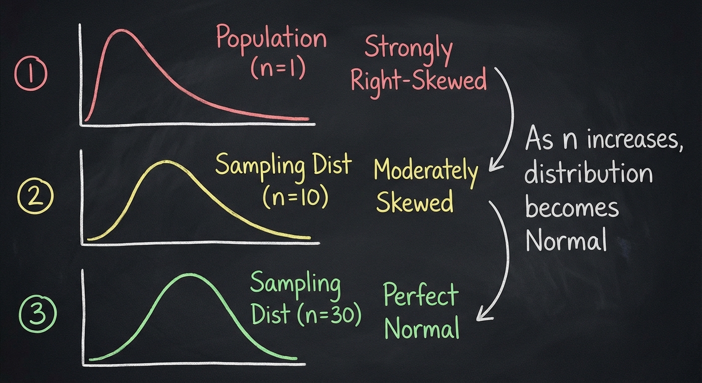
- Case B: The population is not Normal (skewed or uniform), but the sample size is large. This brings us to the most famous theorem in statistics.
The Central Limit Theorem (CLT)
The Central Limit Theorem is the magic that allows us to perform inference even when the population data is messy or skewed.
Definition
The CLT states: If the sample size is large enough ($n \ge 30$), the sampling distribution of the sample mean ($\bar{x}$) will be approximately Normal, regardless of the shape of the population distribution.
Key Nuances of CLT
- It applies to Means, not Proportions. (Proportions use the Large Counts condition).
- It talks about Shape. The CLT tells us the shape becomes Normal. It does not dictate the center or spread.
- The Magic Number is 30. In AP Statistics, $n \ge 30$ is the threshold to satisfy the CLT.
Summary Table: Means vs. Proportions
| Feature | Proportions (Categorical) | Means (Quantitative) |
|---|---|---|
| Statistic | $\hat{p}$ | $\bar{x}$ |
| Parameter | $p$ | $\mu$ |
| Center | $\mu_{\hat{p}} = p$ | $\mu_{\bar{x}} = \mu$ |
| Spread (SD) | $\sqrt{\frac{p(1-p)}{n}}$ | $\frac{\sigma}{\sqrt{n}}$ |
| Normality Condition | Large Counts: $np \ge 10$ AND $n(1-p) \ge 10$ | CLT: Population is Normal OR $n \ge 30$ |
Common Mistakes & Pitfalls
Confusing the Population with the Sampling Distribution
- Mistake: Thinking that if the sample size increases, the population becomes Normal.
- Correction: The population never changes. Only the sampling distribution (the graph of all possible $\bar{x}$'s) becomes Normal as $n$ increases.
Misapplying the Law of Large Numbers (LLN) vs. CLT
- LLN says: As $n$ increases, $\bar{x}$ gets closer to $\mu$ (deals with precision/center).
- CLT says: As $n$ increases, the shape of the distribution of $\bar{x}$ becomes Normal (deals with shape).
Forgetting the Square Root
- When calculating Z-scores for a sampling distribution, students often divide by $\sigma$ instead of the standard deviation of the statistic $\frac{\sigma}{\sqrt{n}}$.
- Wrong Z-score: $z = \frac{\bar{x} - \mu}{\sigma}$
- Correct Z-score: $z = \frac{\bar{x} - \mu}{\sigma / \sqrt{n}}$
Mixing up Normality Conditions
- Do not check "nxp $\ge$ 10" for Means questions.
- Do not check "n $\ge$ 30" for Proportion questions.
Notation Errors
- Using Greek letters ($p, \mu$) for sample statistics.
- Using English letters ($\hat{p}, \bar{x}$) for population parameters.
- Tip: Greek = Parameter (Population). English = Statistic (Sample).