Mastering Confidence Intervals for Means (Unit 7)
Introduction to t-Distributions
When we transition from inference about proportions to inference about means, we encounter a significant hurdle: we rarely know the true population standard deviation ($\sigma$). Because $\sigma$ is unknown, we cannot use the standard normal ($z$) distribution. Instead, we estimate $\sigma$ using the sample standard deviation ($s$) and use the Student’s t-distribution.
Properties of the t-Distribution
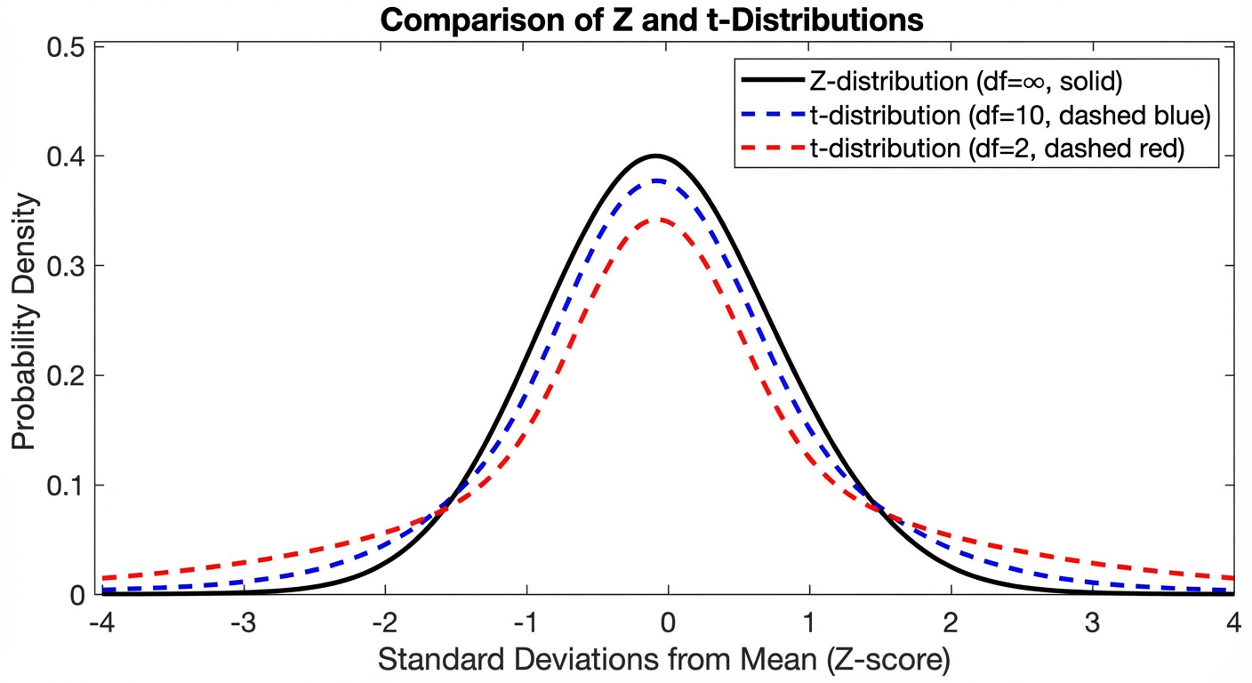
The $t$-distribution is symmetric and bell-shaped, much like the standard normal curve, but it has distinct differences due to the added uncertainty of estimating $\sigma$ with $s$.
- Heavier Tails: The tails are thicker and the peak is lower than the standard normal curve. This reflects the greater variability/uncertainty.
- Degrees of Freedom ($df$): The shape of the distribution depends on the sample size. We define it by degrees of freedom, usually calculated as $df = n - 1$.
- Convergence: As the sample size ($n$) increases (and thus $df$ increases), $s$ becomes a better estimate of $\sigma$, and the $t$-distribution approaches the standard Normal ($z$) distribution.
Determining the Critical Value ($t^*$)
To construct a confidence interval, you need a critical value based on your confidence level (C%) and degrees of freedom.
- Notation: $t^*_{df}$
- Using a Table: Look up the row for your $df$ and the column for your confidence level.
- Using Technology:
invT(area, df)(Remember: for a 95% CI, the "area" to the left is 0.975).
Constructing a Confidence Interval for a Population Mean
This process allows us to estimate the true mean ($\mu$) of a single population based on a sample mean ($\bar{x}$).
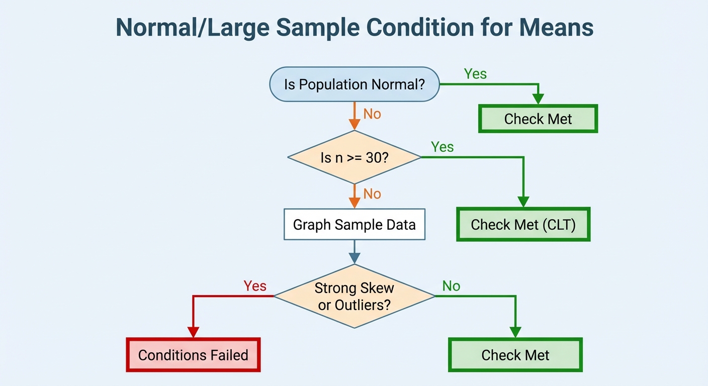
Step 1: Check Conditions
Before calculating, you must verify three conditions (often remembered via the acronym SIN or RIN):
- Random: The data must come from a well-designed random sample or randomized experiment.
- Independence (10% Condition): If sampling without replacement, the sample size ($n$) must be less than 10% of the population size ($N$). ($n \le 0.10N$).
- Normal/Large Sample:
- If the population is known to be Normal: Condition met.
- If $n \ge 30$ (Central Limit Theorem): Condition met.
- If $n < 30$: You must graph the sample data (dot plot or box plot). If there is no strong skewness and no outliers, the condition is met.
Step 2: The Formula
The general structure of a confidence interval is:
For a single mean, the specific formula is (One-sample t-interval):
- $\bar{x}$: Sample mean
- $t^*$: Critical value for $df = n - 1$
- $s$: Sample standard deviation
- $n$: Sample size
- $\frac{s}{\sqrt{n}}$: Standard Error of the mean ($SE_{\bar{x}}$)
Worked Example
Scenario: A coffee shop owner wants to estimate the average weight of their "16 oz" coffee bags. They randomly sample $n=16$ bags, finding a mean weight $\bar{x} = 15.8$ oz with a standard deviation $s = 0.4$ oz. A dot plot of the data shows no strong skew or outliers. Construct a 95% confidence interval.
Solution:
- Conditions: Random (stated), 10% (assume >160 bags exist), Normal (graph check passed).
- Parameters: $df = 16 - 1 = 15$. For 95% confidence, $t^* \approx 2.131$.
- Calculation:
- Conclusion: We are 95% confident that the true mean weight of all coffee bags is between 15.59 and 16.01 oz.
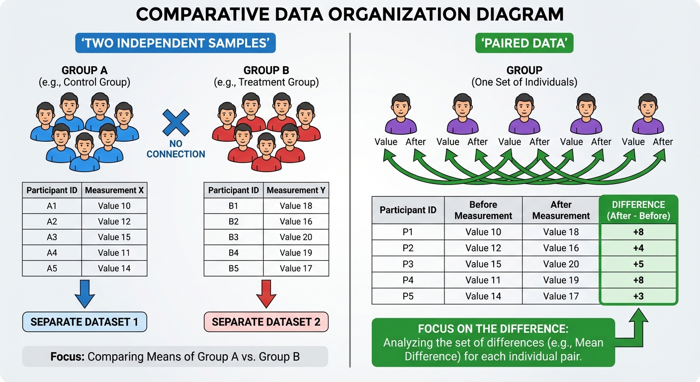
Confidence Interval for a Difference of Two Means
Use this when comparing the means of two independent groups (e.g., Average height of men vs. women).
Conditions for Two Samples
checks must be performed for both groups independently:
- Random: Both samples are independent random samples or randomized treatments.
- Independence: 10% condition checks for both populations (if sampling).
- Normal/Large Sample: $n1 \ge 30$ AND $n2 \ge 30$, or checks on distribution shapes for both samples.
The Formula (Two-Sample t-Interval)
We are estimating the difference in population means $\mu1 - \mu2$.
- Standard Error: $\sqrt{\frac{s1^2}{n1} + \frac{s2^2}{n2}}$
- Degrees of Freedom: There are two methods in AP Statistics.
- Calculator Method (Preferred): The Welch-Satterthwaite formula (messy, requires technology). It yields a decimal $df$ (e.g., $df = 34.6$).
- Conservative Method: Use the smaller of the two simple degrees of freedom: $df = \min(n1 - 1, n2 - 1)$.
Note: Do NOT pool the standard deviations (Method used in Analysis of Variance, not typically for Two-Sample t-intervals in AP Stats).
Interpreting the Difference
When the interval calculates a difference (Group 1 - Group 2):
- Interval includes 0: There is no convincing evidence of a difference in means.
- Interval is entirely positive: Group 1 mean is likely higher.
- Interval is entirely negative: Group 2 mean is likely higher.
Special Case: Paired Data (Matched Pairs)
Often students confuse "Difference of Means" (above) with "Mean Difference" (Paired t-interval).
- Scenario: Pre-test vs. Post-test on the same students; Left arm vs. Right arm; Husband vs. Wife.
- Method: These are NOT independent. You must calculate the difference for each pair ($diff = x2 - x1$) first.
- Analysis: Treat the list of differences as a One-Sample t-Interval where the data is $d1, d2, …$ and you find $\bar{x}{diff}$ and $s{diff}$.
Common Mistakes & Pitfalls
- Using $z$ instead of $t$: If you are using $s$ (sample standard deviation), you MUST use $t$. Only use $z$ if you know the population $\sigma$ (which is rare).
- Incorrect Normal Justification: Saying "Condition met because sample is large" when $n=15$. If $n < 30$, you must reference the shape of the sample distribution (no skew/outliers).
- Confusing Independent vs. Paired:
- Is there a natural link between the two lists of numbers? (e.g., same person, twins). If yes $\to$ Paired t-interval.
- Are the groups totally separate? $\to$ Two-sample t-interval.
- Pooling variances: In AP Stats, we generally select "Pooled: No" on the calculator for Means confidence intervals.
- Interpreting the Interval (Review): Do not say "There is a 95% probability the mean is in the interval." Say "We are 95% confident the interval captures the true mean."