Unit 3: National Income and Price Determination
Aggregate Demand (AD)
Aggregate Demand is the total demand for all final goods and services in an economy at a given time and at various price levels. It represents the sum of spending by households, firms, the government, and the foreign sector.
Unlike valid microeconomic demand curves, which look potential substitutes, the AD curve represents the entire economy—there are no substitutes for "everything."
Determining Aggregate Demand
The formula for Aggregate Demand is identical to the expenditure approach for calculating GDP:
Where:
- $C$ = Consumer Spending (Consumption)
- $I$ = Investment Spending (Gross Private Domestic Investment)
- $G$ = Government Spending
- $(X - M)$ = Net Exports (Exports minus Imports)
The AD Curve Slope
The AD curve is downward sloping, indicating an inverse relationship between the Price Level (PL) and Real GDP demanded.

There are three specific reasons for this downward slope (it is NOT due to the law of diminishing marginal utility):
- The Real Wealth Effect: When the price level falls, the purchasing power of assets (like cash in your wallet or bank account) increases. People feel "wealthier" and therefore buy more goods and services.
- The Interest Rate Effect: When the price level rises, consumers need more money to buy the same amount of goods. This increases the demand for money, which drives up interest rates. Higher interest rates discourage business investment ($I$) and interest-sensitive consumption (like buying cars or homes).
- The Exchange Rate Effect: If the domestic price level rises relative to foreign countries, domestic goods become more expensive to foreigners (Exports fall), and foreign goods become cheaper to domestic consumers (Imports rise). This causes Net Exports to decrease.
Shifting the AD Curve
A change in the Price Level causes a movement along the curve. A change in any component of AD ($C, I, G, X_n$) shifts the entire curve.
- Right Shift (Increase in AD): High consumer confidence, lower taxes, increased government spending, lower interest rates (monetary policy).
- Left Shift (Decrease in AD): Recessions in trading partner countries (lowers exports), decreased wealth (stock market crash), cuts in government spending.
The Multiplier Effect
When the government or consumers change their spending, it ripples through the economy. One person's spending becomes another person's income, leading to further spending. This is the Multiplier Effect.
Marginal Propensities
To understand multipliers, you must understand how households split their disposable income.
- Marginal Propensity to Consume (MPC): The fraction of an additional dollar of income that is spent.
- Marginal Propensity to Save (MPS): The fraction of an additional dollar of income that is saved.
Multiplier Formulas
There are two primary multipliers you need to memorize for the AP exam:
The Spending Multiplier: Used for changes in Government Spending ($G$), Investment ($I$), or autonomous Consumption.
The Tax Multiplier: Used when the government changes lump-sum taxes. Note that this is always negative (taxes up = GDP down) and its absolute value is always smaller than the spending multiplier.
Key Rule: The Balanced Budget Multiplier (increasing $G$ and Taxes determines by the same amount) is always 1. This means if the government taxes you $10B and spends that $10B, GDP rises by exactly $10B.
Example Scenario
Assume the $MPC = 0.8$. Therefore, $MPS = 0.2$.
- Spending Multiplier: $1 / 0.2 = 5$.
- Tax Multiplier: $-0.8 / 0.2 = -4$.
If the government spends $100 million:
Short-Run Aggregate Supply (SRAS)
Aggregate Supply is the total production of goods and services available in an economy at different price levels.
Sticky Wages and Prices
The SRAS curve is upward sloping. This represents a direct relationship between Price Level and Real GDP supplied.
Why is it upward sloping?
It relies on the theory of Sticky Wages (or Sticky Input Prices). In the short run, wages and resource prices are slow to adjust to inflation due to labor contracts and menu costs.
- Scenario: If the Price Level rises (selling price of goods goes up) but wages (cost of labor) stay the same due to contracts, firms make higher profits per unit. This incentivizes them to produce more output.
Shifting the SRAS Curve
Changes in Price Level cause movement along the curve. Shifters of SRAS move the curve. Remember the mnemonic RAP:
- R — Resource Prices (Input Costs): If the price of oil, labor (wages), or raw materials goes up, SRAS shifts left (decreases). This is often called a "Negative Supply Shock."
- A — Actions of Government:
- Taxes: Higher corporate taxes shift SRAS left.
- Subsidies: Subsidies shift SRAS right.
- Regulations: stricter regulations usually increase costs and shift SRAS left.
- P — Productivity: Improvements in technology or human capital allow firms to produce more with the same resources, shifting SRAS right.
Long-Run Aggregate Supply (LRAS)
In the long run, all prices and wages are flexible. They adjust fully to inflation. Therefore, changes in the price level do not affect the profit margins of firms in the long run.
The Vertical Curve
The LRAS curve is vertical at the economy's Full Employment Output ($Yf$ or $Y{FE}$). This represents the potential GDP when the economy is utilizing all resources efficiently (Natural Rate of Unemployment).

Relationship to the PPC
The LRAS curve represents the same concept as the Production Possibilities Curve (PPC). If the PPC shifts outward, the LRAS shifts to the right.
Shifters of LRAS:
Anything that changes the capacity of the economy to produce (Factors of Production):
- New Technology.
- Quantity of Capital (Physical or Human).
- Quantity of Labor (Immigration/Population growth).
- Discovery of new natural resources.
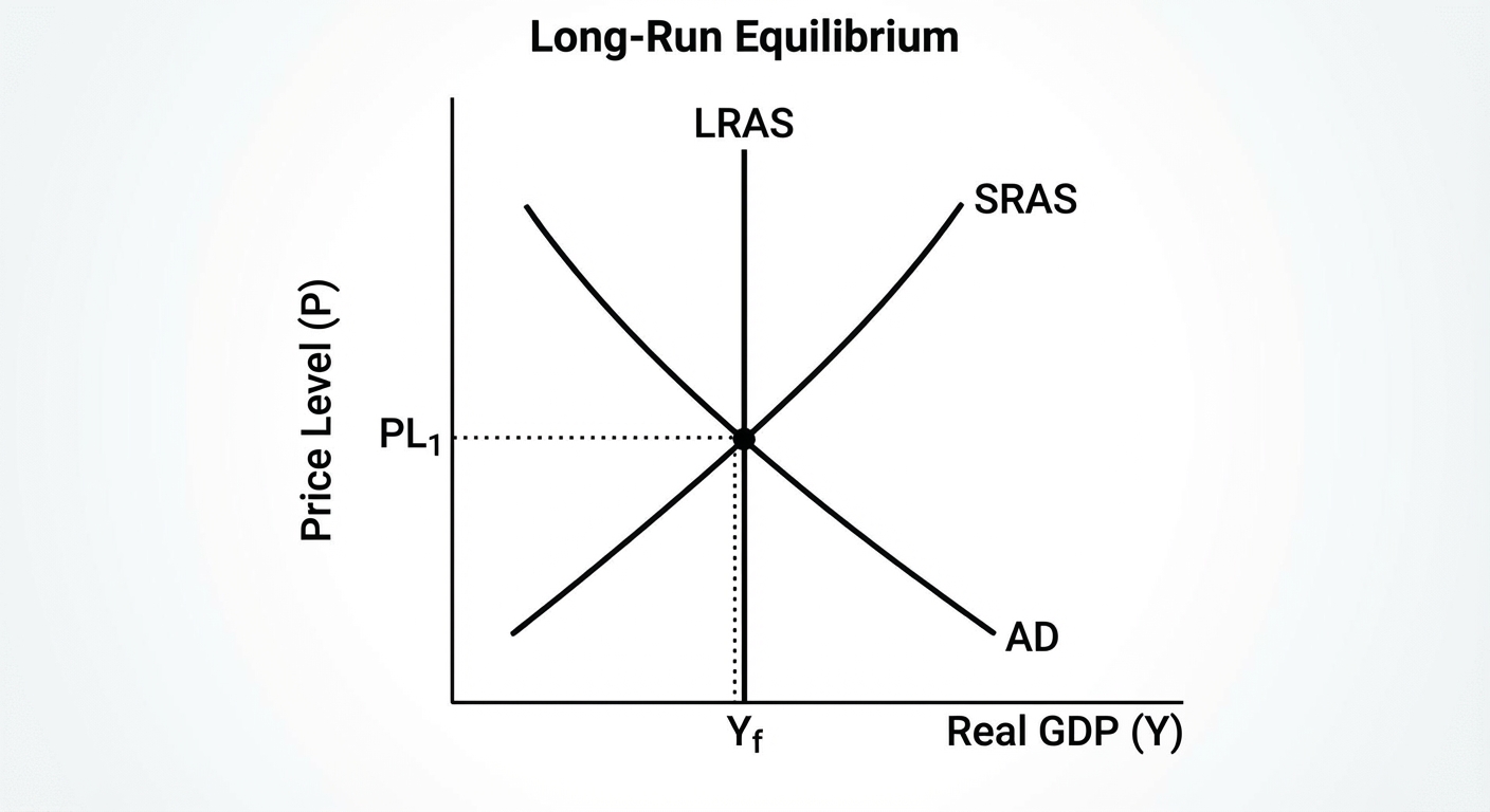
Equilibrium
Putting it all together, the intersection of AD and SRAS determines the equilibrium Price Level and Real GDP. Where all three intersect (AD, SRAS, LRAS), the economy is in long-run equilibrium.
Common Mistakes & Pitfalls
Confusing the "Interest Rate Effect" with Monetary Policy: The Interest Rate Effect explains why the AD curve slopes downward (Price Level $\uparrow$ $\rightarrow$ Demand for Money $\uparrow$ $\rightarrow$ Interest Rates $\uparrow$ $\rightarrow$ GDP $\downarrow$). Do not confuse this with the Federal Reserve changing interest rates, which causes the AD curve to shift.
Spending vs. Tax Multiplier Magnitude: Students often forget that the Spending Multiplier is mathematically stronger than the Tax Multiplier. Government spending hits the economy immediately; tax cuts are partly saved (determined by the MPS) before the rest is spent.
Wages as a Shifter: Remember that wages affect SRAS, not AD. While wages are income for consumers (potentially affecting C), in the AS/AD model, widespread wage changes are treated primarily as a change in input costs for firms, shifting SRAS.
Short Run vs. Long Run: Always check if the question asks for the immediate impact (SRAS shifts, Price Level changes) or the long-run adjustment (wages adjust, SRAS shifts back to restore Full Employment).