Unit 6 Review: Inference for Categorical Data and Proportions
Introduction to Significance Tests and Setting Up Hypotheses
Statistical inference allows us to make judgments about population parameters based on sample data. A significance test (or hypothesis test) is a formal procedure for comparing observed data with a claim (hypothesis) whose truth we want to assess.
The Logic of Hypothesis Testing
The logic follows a "proof by contradiction" model, similar to a criminal trial. We start by assuming the null hypothesis is true, then we examine the evidence (data). If the evidence is incredibly unlikely to occur under that assumption, we reject the assumption.
Defining the Hypotheses
Every test requires two competing hypotheses stated in terms of population parameters (like $p$), never sample statistics (like $\hat{p}$).
- Null Hypothesis ($H_0$): The claim of "no difference," "no effect,” or the status quo. It always includes an equality sign ($=$, $\leq$, or $\geq$).
- Format: $H0: p = p0$ (where $p_0$ is the hypothesized value).
- Alternative Hypothesis ($H_a$): The claim we hope or suspect is true. It looks for evidence against the null.
- One-sided (left): $Ha: p < p0$ (checking for a decrease)
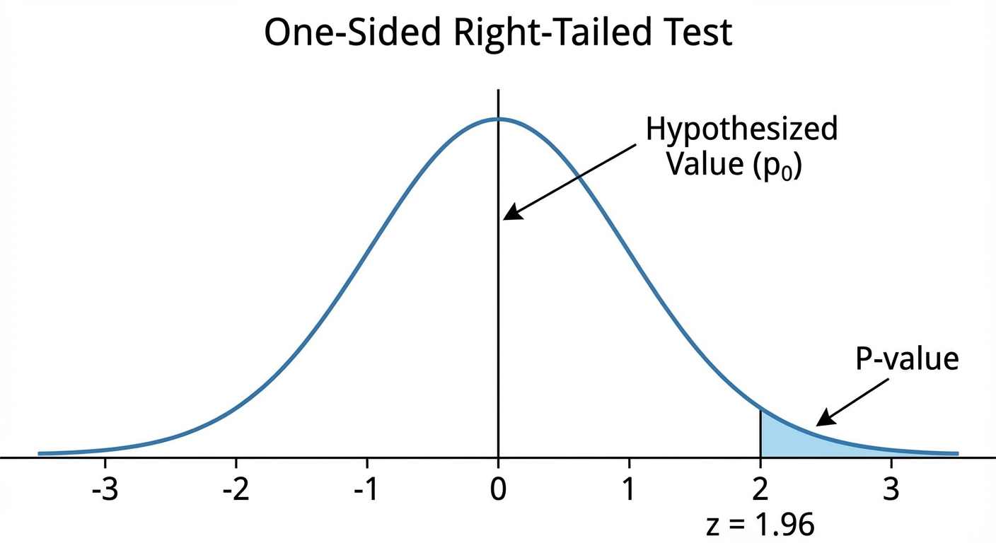
- One-sided (right): $Ha: p > p0$ (checking for an increase)
- Two-sided: $Ha: p \neq p0$ (checking for any difference)
P-Values and Significance Levels
To make a decision, we compare the P-value to a significance level, denoted by alpha ($\alpha$).
- P-value: The probability of obtaining a test statistic as extreme as, or more extreme than, the observed statistic, assuming $H_0$ is true.
- Small P-value: Strong evidence against $H_0$.
- Large P-value: Weak evidence against $H_0$.
- Significance Level ($\alpha$): The threshold for rejection (commonly 0.05, 0.01, or 0.10).
Decision Rule:
- If $P\text{-value} \leq \alpha \rightarrow$ Reject $H_0$. (The result is statistically significant).
- If $P\text{-value} > \alpha \rightarrow$ Fail to reject $H_0$. (Insufficient evidence).
Carrying Out a Significance Test for a Population Proportion
When testing a claim about a single proportion, we use the One-Sample $z$-Test for a Proportion. On the AP exam, you must follow the "State, Plan, Do, Conclude" format.
Step 1: State
Clearly state the hypotheses ($H0$ and $Ha$) and define the parameter $p$ in the context of the problem.
Step 2: Plan
Identify the inference method (One-sample $z$-test for $p$) and verify the conditions:
- Random: The data comes from a random sample or randomized experiment.
- Independence (10% Condition): If sampling without replacement, sample size $n \leq \frac{1}{10}N$ (population size).
- Large Counts: This ensures the sampling distribution is approximately Normal.
- Crucial difference from Confidence Intervals: We assume $H0$ is true, so we use the null parameter value $p0$, not $\hat{p}$.
- Check: and .
Step 3: Do
Calculate the test statistic and finding the P-value.
The Test Statistic ($z$):
This measures how many standard deviations the sample proportion $\hat{p}$ is from the null value $p_0$.
Note: The denominator uses $p0$, not $\hat{p}$, because standard deviation is calculated assuming $H0$ is true.
Finding the P-value:
Use a Standard Normal Table ($z$-table) or technology (normalcdf) to find the probability associated with the calculated $z$-score based on the direction of $H_a$.
Step 4: Conclude
Compare the P-value to $\alpha$. Write a sentence in context:
"Because the P-value of [value] is [less/greater] than $\alpha = 0.05$, we [reject/fail to reject] the null hypothesis. There [is/is not] convincing evidence that [restate $H_a$ in context]."
Type I and Type II Errors and Power
We can never be 100% certain in statistics. Even when we follow the procedure perfectly, sampling variability can lead to incorrect conclusions.
Error Types
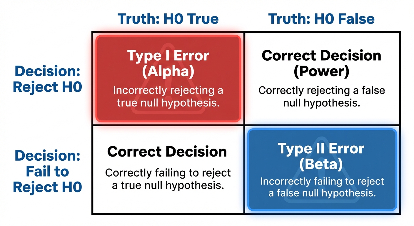
| $H_0$ is True | $H0$ is False ($Ha$ is True) | |
|---|---|---|
| Reject $H_0$ | Type I Error (False Positive) | Correct Decision (Power) |
| Fail to Reject $H_0$ | Correct Decision | Type II Error (False Negative) |
- Type I Error: Rejecting $H_0$ when it is actually true.
- The probability of a Type I error is exactly the significance level: .
- Type II Error: Failing to reject $H_0$ when it is actually false.
- The probability is denoted by $\beta$ (beta).
Power of a Test
Power is the probability that the test correctly rejects a false null hypothesis.
How to Increase Power:
To detect a difference from the null more easily, you can:
- Increase Sample Size ($n$): This reduces standard deviation, making the distribution narrower and easier to distinguish.
- Increase $\alpha$: Making it easier to reject $H_0$ increases Power (but also increases the risk of Type I error).
- Effect Size: If the true parameter is very far from $p_0$, it is easier to detect.
Mnemonic: "The Boy Who Cried Wolf"
- Null Hypothesis: There is no wolf.
- Type I Error: The boy cries wolf when there is none (False Alarm). The village loses trust (Cost of error).
- Type II Error: The boy stays silent when there is a wolf (Missed Detection). The sheep get eaten (Cost of error).
Confidence Intervals and Tests for the Difference of Two Proportions
When comparing proportions from two distinct populations (e.g., "Do a higher proportion of teens like TikTok than adults?"), we use a two-sample $z$-test.
Hypothesis Setup
- $H0: p1 - p2 = 0$ (OR $p1 = p_2$)
- $Ha: p1 - p_2 \neq 0$ (or $
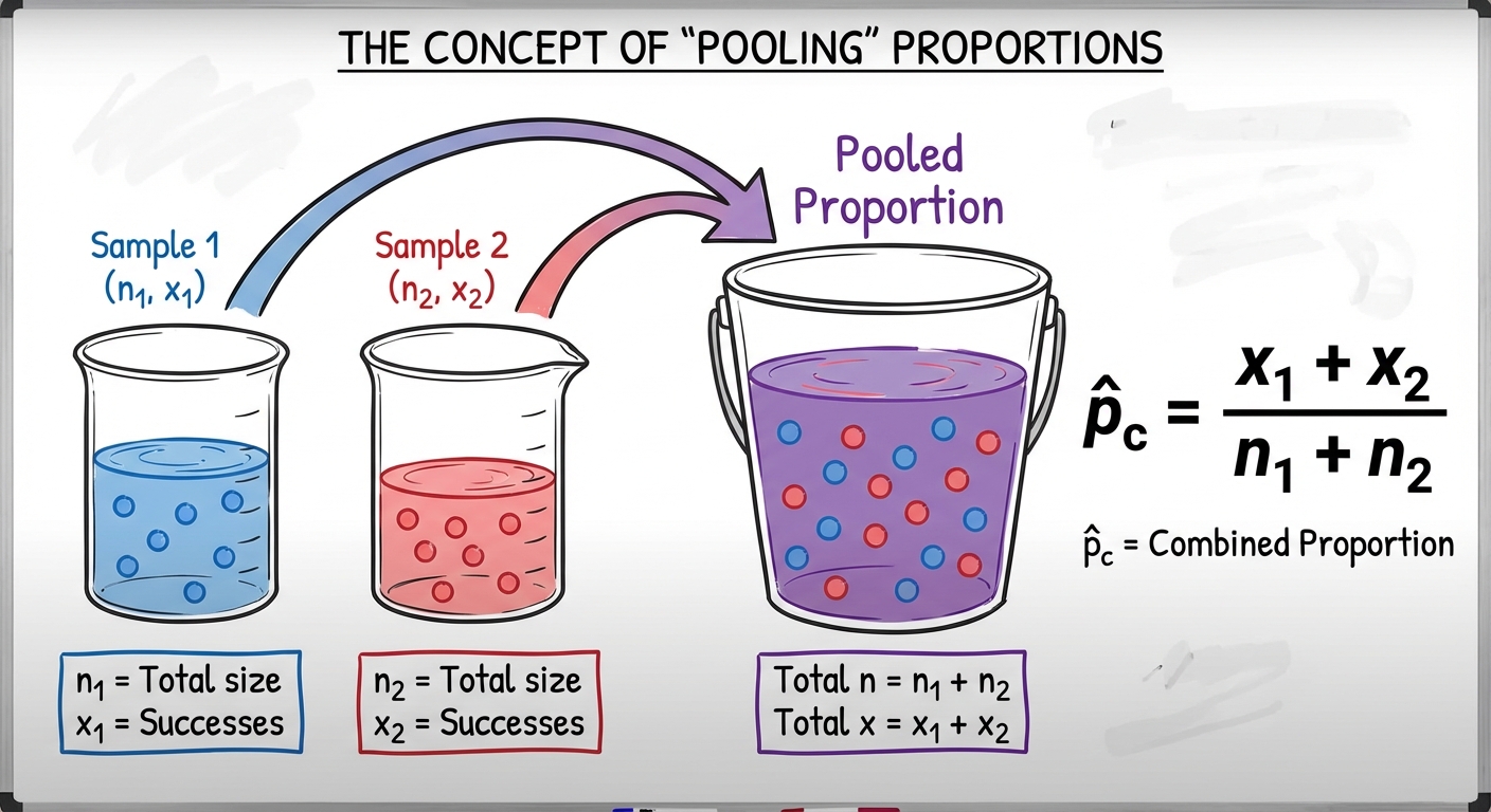
Pooling: The Key Difference
This is the most frequent conceptual hurdle.
- For Confidence Intervals: We do NOT assume $p1 = p2$. We estimate standard error using the individual sample proportions $\hat{p}1$ and $\hat{p}2$.
- For Significance Tests: We assume $H0$ is true, meaning $p1 = p_2$. If the populations are the same, we should combine the data to get a better estimate of the "common" proportion.
The Combined (Pooled) Proportion $\hat{p}c$:
The Two-Sample $z$-Test Statistic
Conditions for Two-Sample Tests
- Random: Two independent random samples or randomized treatments.
- Independence (10%): $n1 < 0.10N1$ and $n2 < 0.10N2$.
- Large Counts: Counts of successes and failures in both samples must be $\geq 10$.
- Technically, since we pool, you can check $n1\hat{p}c$, $n1(1-\hat{p}c)$, etc., but checking observed counts $x1, n1-x_1$ (success/failures) is generally accepted on the AP exam for two-sample tests.
Relationship Between CI and Tests
A Confidence Interval provides more information than a test.
- If the $95\%$ confidence interval for $p1 - p2$ does not include 0, it is equivalent to rejecting $H0: p1 - p_2 = 0$ at the $\alpha = 0.05$ level (for a two-sided test).
- If the interval includes 0, we fail to reject $H_0$.
Common Mistakes & Pitfalls
- Hypotheses Notation Errors: AVOID writing $H_0: \hat{p} = 0.5$. Hypotheses are always about parameters ($p$), never statistics ($\hat{p}$).
- Accepting the Null: NEVER conclude "We accept $H0$." We only "Fail to reject $H0$." (Think: "Not guilty" implies we didn't have enough evidence to convict, not that the defendant is definitely innocent).
- Using $\hat{p}$ in One-Sample Standard Error: In a one-sample test, you must use $p_0$ inside the square root denominator. In a confidence interval, you use $\hat{p}$.
- Forgetting to Pool: In a two-sample test for proportions involving $H0: p1 = p2$, you must use the pooled proportion $\hat{p}c$ for the standard error.
- Large Counts Confusion:
- One-Sample Test: Use $n p_0$.
- One-Sample Interval: Use $n \hat{p}$.