AP Calculus AB Unit 5 Study Guide: Analytical Applications of Differentiation
The Mean Value Theorem Family: What Derivatives Guarantee
Derivatives are often introduced as a rate of change and a slope of the tangent line. In Unit 5, you lean into a deeper idea: derivatives can also be used to prove that certain events must happen somewhere on an interval. The big theorems in this unit (Extreme Value Theorem, Rolle’s Theorem, Mean Value Theorem) are “existence” results. They usually do not tell you where something happens right away, but they guarantee that it happens at least once.
A key theme is that these theorems require specific conditions, especially continuity on a closed interval and differentiability on the open interval. Many AP questions are really condition-checking questions in disguise: if the hypotheses are not met, you cannot conclude the theorem’s guarantee.
Continuity vs. differentiability (and why the distinction matters)
A function is continuous at a point if you can draw its graph there without lifting your pencil. More formally, the limit equals the function value. Continuity is about whether the function has “breaks” (holes, jumps, vertical asymptotes).
A function is differentiable at a point if it has a derivative there. Geometrically, that means it has a well-defined tangent slope. Differentiability is stricter than continuity: if a function is differentiable at a point, it must be continuous there, but a function can be continuous and still fail to be differentiable (corners, cusps, vertical tangents).
This matters because theorems about attaining max/min values require continuity, while theorems connecting average rate of change to instantaneous rate of change require both continuity and differentiability.
Mean Value Theorem (MVT)
The Mean Value Theorem is one of the most important existence theorems in calculus. It connects the average rate of change over an interval to the instantaneous rate of change at some interior point.
Hypotheses (conditions): If %%LATEX0%% is continuous on %%LATEX1%% and differentiable on , then the theorem applies.
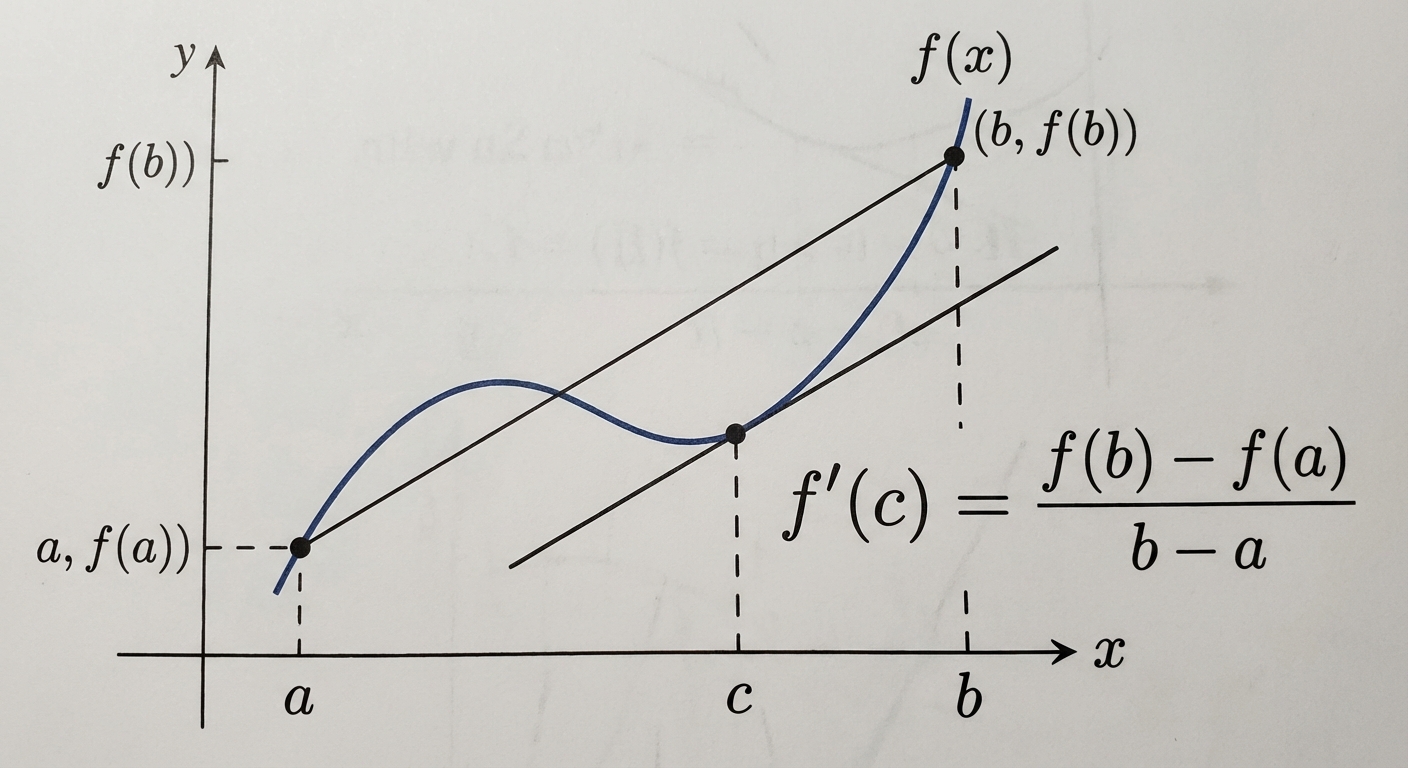
Conclusion: There exists at least one number %%LATEX3%% with %%LATEX4%% such that:
The right-hand side is the slope of the secant line from %%LATEX6%% to %%LATEX7%%, which is the average rate of change. The theorem guarantees that somewhere between %%LATEX8%% and %%LATEX9%% there is a tangent line parallel to that secant line.
A common real-world interpretation uses motion: if you drive from point A to point B and your average speed is 50 mph, then at some instant your speedometer read exactly 50 mph (under the idealized assumption your position function is continuous and differentiable).
Worked example
Let %%LATEX10%% on %%LATEX11%%.
First, %%LATEX12%% is a polynomial, so it is continuous on %%LATEX13%% and differentiable on .
Compute average rate of change:
Now solve . Since:
we get:
Rolle’s Theorem
Rolle’s Theorem is a special case of MVT where the starting and ending values match.
If %%LATEX20%% is continuous on %%LATEX21%%, differentiable on %%LATEX22%%, and %%LATEX23%%, then there exists at least one number %%LATEX24%% in %%LATEX25%% such that:
Translation: somewhere between two points with the same height, the graph must “flatten out” (have a horizontal tangent).
Worked example
Let %%LATEX27%% on %%LATEX28%%.
Polynomials are continuous and differentiable everywhere. Compute endpoint values:
Because %%LATEX31%%, Rolle’s Theorem applies. Now find %%LATEX32%% where .
Since %%LATEX37%% is in %%LATEX38%%, it satisfies the theorem.
How Rolle’s Theorem fits inside MVT
Rolle’s Theorem is exactly MVT when the secant slope is zero. If , then:
so MVT becomes “there exists %%LATEX41%% with %%LATEX42%%.”
Extreme Value Theorem (EVT)
The Extreme Value Theorem guarantees the existence of absolute extrema.
If %%LATEX43%% is continuous on a closed interval %%LATEX44%%, then %%LATEX45%% attains (actually reaches) both an absolute maximum value and an absolute minimum value on %%LATEX46%%.
“Attains” matters: it means there exists at least one input where the max happens and at least one input where the min happens.
Why the conditions matter: the interval must be closed because absolute extrema may occur at endpoints, and the function must be continuous because otherwise it might approach a value without ever reaching it. EVT does not tell you where the extrema occur, and it does not say they are unique.
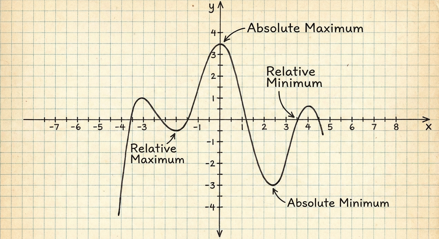
Local (relative) vs. absolute (global)
Absolute extrema are the highest or lowest -values on the entire domain or interval. Relative extrema are the highest or lowest values compared only to nearby points (the “hills and valleys” idea).
Example: EVT can fail if the interval is not closed
Consider %%LATEX48%% on %%LATEX49%%. The function is continuous there, but the interval is not closed. As %%LATEX50%% approaches %%LATEX51%% from the right, %%LATEX52%% grows without bound, so there is no absolute maximum on %%LATEX53%%.
Example: EVT can fail if the function is not continuous
Consider a function with a hole at the top “peak.” If the function approaches a highest value but the point is missing, the absolute maximum does not exist.
Exam Focus
Typical question patterns include: “Does the Mean Value Theorem apply on %%LATEX54%%? Justify.” (You must explicitly state continuity on %%LATEX55%% and differentiability on %%LATEX56%%.) Another standard prompt is “Find all values of %%LATEX57%% guaranteed by the MVT,” which means compute the secant slope and solve %%LATEX58%%, then confirm %%LATEX59%% lies in . You may also be asked to use Rolle’s Theorem or MVT as a reasoning tool to prove that a certain derivative value occurs.
Common mistakes include forgetting that differentiability is required on the open interval, not the closed one; assuming “it looks smooth” is a valid justification when the function is piecewise or has a known issue; and solving for a %%LATEX61%% that is not in %%LATEX62%%.
Critical Points and the First Derivative: Increasing, Decreasing, and Extrema
Once you can compute derivatives, you can use them as an analysis tool rather than just a slope calculator. The sign of the derivative tells you how the function behaves.
Increasing and decreasing behavior
If %%LATEX63%% is positive, the function is increasing there. Over an interval, you use the sign of %%LATEX64%%:
If %%LATEX65%% for every %%LATEX66%% in an interval, then %%LATEX67%% is increasing on that interval. If %%LATEX68%% for every %%LATEX69%% in an interval, then %%LATEX70%% is decreasing on that interval.
Critical points (where “something can happen”)
A critical point (or critical number) of a function %%LATEX71%% is a number %%LATEX72%% in the domain of such that either:
or does not exist.
Critical points matter because local maxima and minima can occur only at critical points (or at endpoints when you are looking for absolute extrema on a closed interval). Not every critical point is an extremum, but you only need to check critical points.
Common sources of critical points include horizontal tangents, corners/cusps, and vertical tangents. A subtle but important point is that a discontinuity is not automatically a critical point because the definition requires %%LATEX76%% to be in the domain of %%LATEX77%%.
The Number Line Test (sign chart procedure)
A reliable way to decide where a function increases or decreases is the number line test:
- Find the domain of .
- Compute and determine all critical points.
- Place critical points on a number line.
- Test a value in each sub-interval in to determine the sign.
Example: Increasing/decreasing via number line test
Let:
Differentiate:
Factor to find critical points:
So critical points are %%LATEX85%% and %%LATEX86%%.
Now test intervals:
For %%LATEX87%% (test %%LATEX88%%):
so is increasing there.
For %%LATEX91%% (test %%LATEX92%%):
so is decreasing there.
For %%LATEX95%% (test %%LATEX96%%):
so is increasing there.
Local (relative) extrema
A local maximum occurs at %%LATEX99%% if %%LATEX100%% is greater than or equal to nearby values. A local minimum occurs if is less than or equal to nearby values.
First Derivative Test (sign change test)
The First Derivative Test classifies a critical point %%LATEX102%% by how %%LATEX103%% changes sign around .
If %%LATEX105%% changes from positive to negative at %%LATEX106%%, then %%LATEX107%% has a local maximum at %%LATEX108%%. If %%LATEX109%% changes from negative to positive at %%LATEX110%%, then %%LATEX111%% has a local minimum at %%LATEX112%%. If %%LATEX113%% does not change sign, then %%LATEX114%% is not a local extremum (it may be a “plateau”).
Applying the First Derivative Test to the example above
At %%LATEX115%%, the sign changes from positive to negative, so %%LATEX116%% is a relative maximum. At %%LATEX117%%, the sign changes from negative to positive, so %%LATEX118%% is a relative minimum.
Example: Analyze increasing/decreasing and local extrema
Let:
Compute derivative:
Factor:
Critical points occur at %%LATEX122%% and %%LATEX123%%.
Sign chart testing shows %%LATEX124%% on %%LATEX125%%, %%LATEX126%% on %%LATEX127%%, and %%LATEX128%% on %%LATEX129%%. Therefore, %%LATEX130%% increases on %%LATEX131%%, decreases on %%LATEX132%%, and increases on %%LATEX133%%.
Since %%LATEX134%% changes from positive to negative at %%LATEX135%%, there is a local maximum there. Since %%LATEX136%% changes from negative to positive at %%LATEX137%%, there is a local minimum there.
Optional values:
Absolute extrema on a closed interval (Closed Interval Method / Candidates Test)
Local extrema are not enough when a problem asks for the absolute maximum or minimum on a closed interval %%LATEX140%%. If %%LATEX141%% is continuous on , EVT guarantees absolute extrema exist.
To find them, use the Closed Interval Method, also commonly called the Candidates Test:
- Confirm %%LATEX143%% is continuous on %%LATEX144%%.
- Find all critical points inside .
- Evaluate %%LATEX146%% at every critical point and at the endpoints %%LATEX147%% and .
- Compare the function values: the largest is the absolute maximum; the smallest is the absolute minimum.
A classic common mistake is forgetting endpoints. The absolute max often occurs at the start or end of the interval, not just at peaks and valleys.
Worked example: Absolute extrema on an interval
Find the absolute maximum and minimum of %%LATEX149%% on %%LATEX150%%.
Critical points are %%LATEX151%% and %%LATEX152%%. Evaluate at endpoints and critical points:
Absolute maximum value is %%LATEX157%% (occurs at %%LATEX158%% and %%LATEX159%%). Absolute minimum value is %%LATEX160%% (occurs at %%LATEX161%% and %%LATEX162%%). This also illustrates that absolute extrema need not be unique.
Exam Focus
Typical question patterns include finding intervals where %%LATEX163%% is increasing or decreasing (compute %%LATEX164%%, find critical points, do sign analysis), finding and classifying local extrema (First Derivative Test), and finding absolute maxima/minima on (Candidates Test).
Common mistakes include treating every solution to %%LATEX166%% as an extremum without checking a sign change, ignoring where %%LATEX167%% does not exist even though does, and forgetting endpoints when asked for absolute extrema.
Concavity, Inflection Points, and the Second Derivative
The first derivative tells you whether the function is going up or down. The second derivative tells you how the slope itself is changing. This is the mathematical version of distinguishing “moving forward” from “speeding up.”
Concavity: what it means geometrically
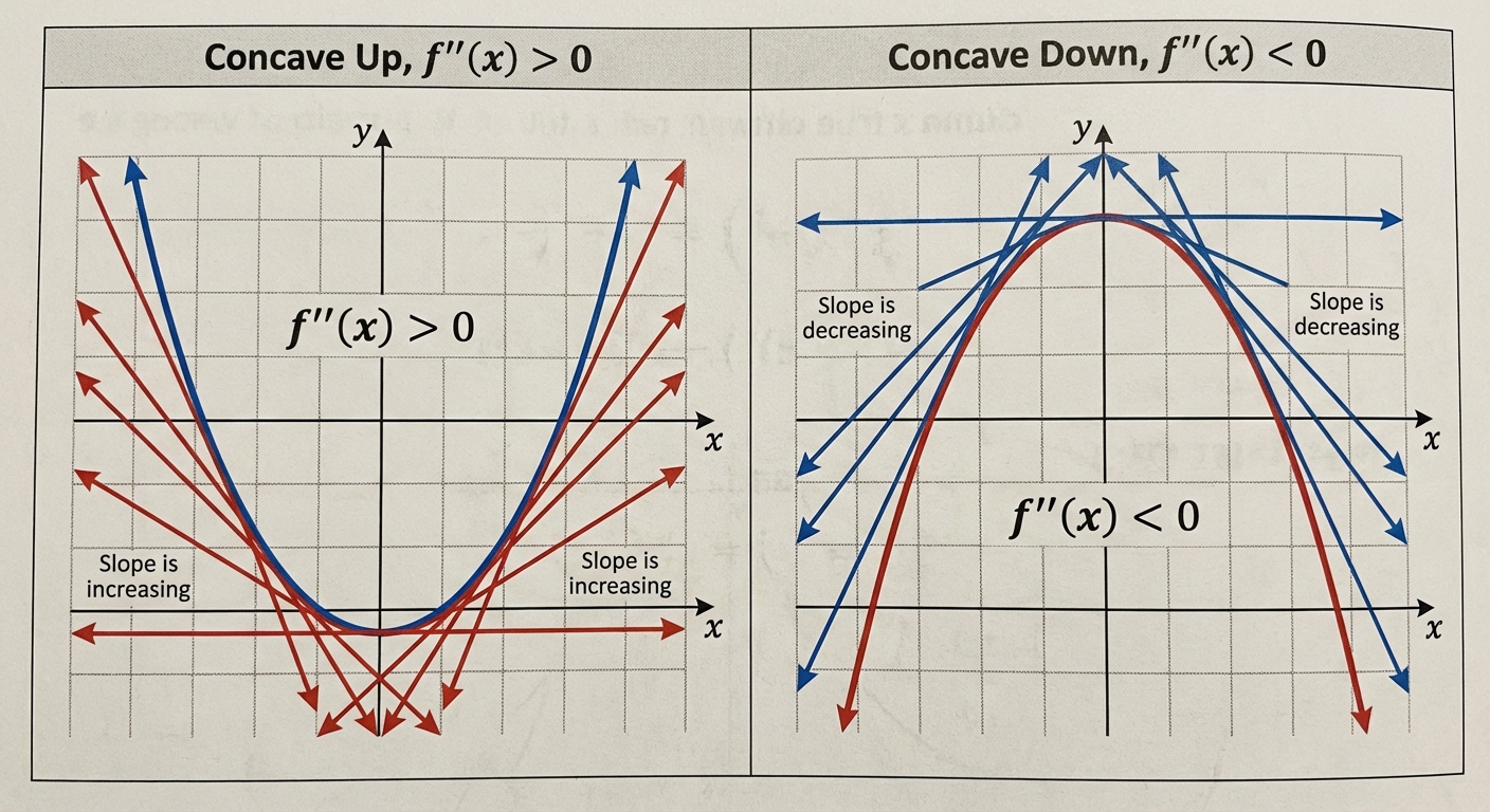
A function is concave up on an interval if it curves like a cup: as you move left to right, the slopes increase. A function is concave down if it curves like a cap: the slopes decrease.
Because %%LATEX169%% measures the rate of change of %%LATEX170%%, you get the standard test:
If %%LATEX171%% on an interval, then %%LATEX172%% is concave up there. If %%LATEX173%% on an interval, then %%LATEX174%% is concave down there.
Inflection points (points of inflection)
An inflection point is a point on the graph where concavity changes (from up to down or down to up).
Possible inflection points occur where %%LATEX175%% or %%LATEX176%% is undefined, but neither condition alone guarantees an inflection point. You must confirm that concavity actually changes, usually by checking a sign change in .
One common classroom checklist says that the tangent line should exist at %%LATEX178%% (or the graph should have a vertical tangent) when naming a point of inflection. The mathematically essential idea for AP Calculus is: the point must be on the graph (so %%LATEX179%% is defined), and concavity must change across .
Example: Concavity and inflection points
Let:
Compute derivatives:
Solve :
Testing shows is concave down on:
and concave up on:
and:
Concavity changes at both values, so both are inflection points.
Example: Point of inflection from a polynomial used in first-derivative analysis
Using the earlier function:
we had:
Now compute the second derivative:
Possible inflection points come from :
Check sign: for %%LATEX198%%, %%LATEX199%% (concave down), and for %%LATEX200%%, %%LATEX201%% (concave up). Since %%LATEX202%% changes sign, %%LATEX203%% is a point of inflection.
Second Derivative Test (classifying a critical point)
The Second Derivative Test can classify a critical point %%LATEX204%% where %%LATEX205%%.
If %%LATEX206%%, then %%LATEX207%% has a local minimum at %%LATEX208%%. If %%LATEX209%%, then %%LATEX210%% has a local maximum at %%LATEX211%%. If , the test is inconclusive, and you should use the First Derivative Test instead.
Mnemonic: if %%LATEX213%% is positive, think “happy face” and a minimum at the bottom. If %%LATEX214%% is negative, think “sad face” and a maximum at the top.
Example: Second derivative test in action
Let:
Critical points occur at %%LATEX216%% and %%LATEX217%%. We already have:
Compute:
Evaluate:
So is a local maximum.
So is a local minimum.
Concavity in real contexts: motion
If is position, then:
If %%LATEX227%%, position is increasing (moving in the positive direction). If %%LATEX228%%, velocity is increasing. If %%LATEX229%% and %%LATEX230%%, you are moving forward and speeding up. If %%LATEX231%% and %%LATEX232%%, you are moving forward but slowing down.
Exam Focus
Typical question patterns include finding intervals of concavity and points of inflection (compute %%LATEX233%%, solve %%LATEX234%%, and verify a sign change), using the second derivative test to classify critical points, and motion interpretation problems linking %%LATEX235%%, %%LATEX236%%, and .
Common mistakes include declaring an inflection point just because %%LATEX238%% without checking concavity change, forgetting that %%LATEX239%% can be undefined at a point where concavity still changes, and mixing up concavity (change in slope) with increasing/decreasing (sign of slope).
Connecting Graphs of %%LATEX240%%, %%LATEX241%%, and (Graphical Analysis)
A major analytical application skill is moving between information about a function and information about its derivatives. On the AP exam, you might be given a graph of %%LATEX243%% and asked about %%LATEX244%%, a graph of %%LATEX245%% and asked where %%LATEX246%% increases or has extrema, or a table of values for %%LATEX247%% or %%LATEX248%% and asked to interpret behavior.
Quick translation table (features across %%LATEX249%%, %%LATEX250%%, )
| Feature of | Behavior of (slope) | Behavior of (concavity) |
|---|---|---|
| Increasing | Positive, above the -axis | N/A |
| Decreasing | Negative, below the -axis | N/A |
| Relative Max | Changes positive to negative (an %%LATEX257%%-intercept of %%LATEX258%%) | Negative (usually) |
| Relative Min | Changes negative to positive (an %%LATEX259%%-intercept of %%LATEX260%%) | Positive (usually) |
| Concave Up | is increasing | Positive, above the -axis |
| Concave Down | is decreasing | Negative, below the -axis |
| Point of Inflection | often has a relative max or min | %%LATEX266%% changes sign (an %%LATEX267%%-intercept of ) |
From %%LATEX269%% to %%LATEX270%%
If you have a graph of %%LATEX271%%, then %%LATEX272%% is increasing where %%LATEX273%% and decreasing where %%LATEX274%%. Critical points of %%LATEX275%% occur where %%LATEX276%% or where %%LATEX277%% is undefined (as long as %%LATEX278%% is defined). A local maximum of %%LATEX279%% occurs where %%LATEX280%% changes from positive to negative, and a local minimum occurs where changes from negative to positive.
From %%LATEX282%% (or the shape of %%LATEX283%%) to concavity of
If you have %%LATEX285%%, then %%LATEX286%% is concave up where %%LATEX287%% and concave down where %%LATEX288%%.
If you only have a graph of %%LATEX289%%, you can still get concavity: %%LATEX290%% is concave up where %%LATEX291%% is increasing, and concave down where %%LATEX292%% is decreasing.
Inflection points from a graph of
Inflection points of %%LATEX294%% happen where concavity changes, which corresponds to %%LATEX295%% changing sign. On a graph of %%LATEX296%%, that often appears where %%LATEX297%% changes from increasing to decreasing or vice versa, meaning has a local maximum or minimum.
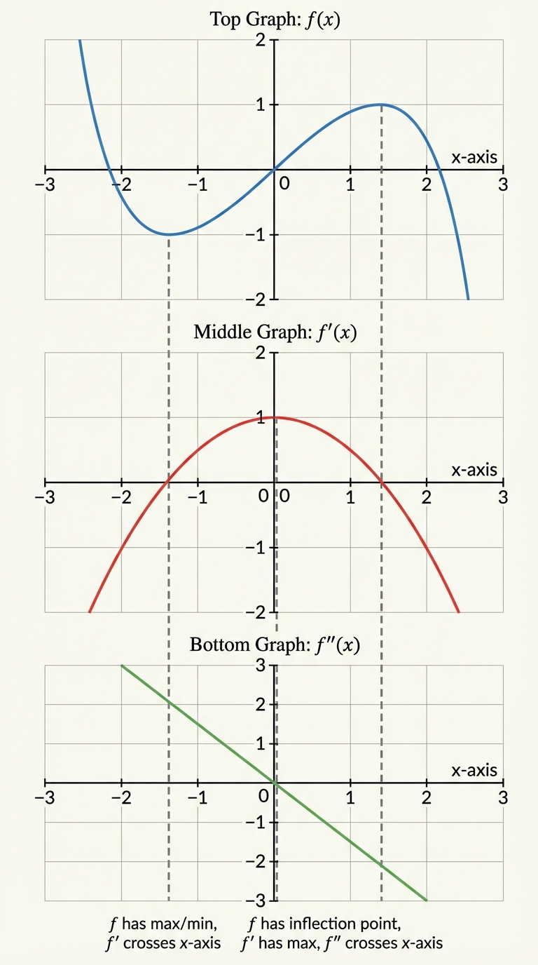
Example: Reading behavior from (conceptual walkthrough)
Suppose you are given a graph of %%LATEX300%% and you observe that %%LATEX301%% crosses the %%LATEX302%%-axis at %%LATEX303%% going from positive to negative, and %%LATEX304%% has a local minimum at %%LATEX305%%. Then %%LATEX306%% has a local maximum at %%LATEX307%%, and %%LATEX308%% has an inflection point at %%LATEX309%%.
“Sketch the graph” with derivative information (what you actually need to do)
When AP asks for a sketch based on derivative information, you are not expected to create perfect artwork. You are expected to show the correct qualitative features: where the function increases or decreases, where it has relative maxima or minima, where it is concave up or down, and where inflection points occur.
Common confusion: critical points vs. inflection points
Critical points of %%LATEX310%% come from %%LATEX311%% or %%LATEX312%% undefined. Inflection points of %%LATEX313%% come from concavity changes, often tested by %%LATEX314%% or %%LATEX315%% undefined together with a sign change.
A very common graph-based error is confusing a feature of %%LATEX316%% with a feature of %%LATEX317%%: if you are looking at the graph of %%LATEX318%%, a maximum of %%LATEX319%% usually corresponds to a point of inflection of %%LATEX320%%, not a maximum of %%LATEX321%%.
Exam Focus
Typical question patterns include using a graph of %%LATEX322%% to find where %%LATEX323%% increases or decreases and where %%LATEX324%% has relative extrema, using a graph or sign chart of %%LATEX325%% and to determine concavity and inflection points, and sketching a possible graph given sign and concavity data.
Common mistakes include saying %%LATEX327%% means inflection point (it does not), reading %%LATEX328%% above the axis as “concave up” instead of “increasing,” and forgetting that a derivative being undefined can create a critical point (if is defined there) and can also matter for concavity changes.
Optimization: Using Derivatives to Choose the Best Option
Optimization problems ask you to maximize or minimize a quantity (area, volume, cost, time, distance, profit, material used) subject to constraints. The calculus is usually straightforward; the challenge is translating words into equations and respecting the feasible domain.
General strategy (a strong AP-friendly workflow)
- Draw a picture and label constants and variables.
- Write the primary equation (objective function) for the quantity you want to maximize or minimize.
- Write a constraint equation relating the variables.
- Use substitution to rewrite the objective function in terms of a single variable.
- Identify the feasible domain, often a closed interval .
- Use calculus: compute the derivative, set it equal to zero, and find critical points.
- Verify max or min using the First Derivative Test, Second Derivative Test, or the Candidates Test if the domain is closed.
- Answer the question in context, including units, and double-check whether it asks for the maximizing/minimizing input value or the resulting dimensions/value.
A common mistake is to do the derivative work correctly but ignore the domain, producing an “optimal” value that is physically impossible (like a negative length).
Why derivatives find maxima and minima in optimization
If an objective function %%LATEX331%% is smooth and has an interior maximum or minimum at %%LATEX332%%, then:
However, the optimum can occur at an endpoint of the feasible domain, so endpoints must be checked when the domain is closed.
Optimization example 1: Maximize area with fixed perimeter
A rectangle has perimeter 100 units. What dimensions maximize its area?
Let side lengths be %%LATEX334%% and %%LATEX335%%. The area is:
The constraint is:
Solve for :
Substitute:
Domain: .
Differentiate:
Set to zero:
Second derivative:
So the critical point is a maximum. Then:
The rectangle with maximum area is a square, %%LATEX347%% by %%LATEX348%%. A useful general principle is that among rectangles with fixed perimeter, the square has the greatest area.
Optimization example 2: Minimize surface area of a closed cylinder with fixed volume
A closed cylinder must hold volume 500 cubic units. Find the radius and height that minimize surface area.
Let radius be %%LATEX349%% and height be %%LATEX350%%.
Surface area (closed cylinder):
Volume constraint:
Given :
Solve for :
Substitute into :
Simplify:
Differentiate:
Set to zero:
Now compute :
Using the relationship above leads to:
So the minimum-surface-area closed cylinder occurs when height equals diameter.
A good reason this critical point is a minimum is end behavior: as %%LATEX368%%, the term %%LATEX369%% becomes huge, and as %%LATEX370%%, the term %%LATEX371%% becomes huge, so a single interior critical point reasonably gives the minimum.
How AP wants optimization written (communication)
In free-response, points are often earned for clearly defining variables, writing correct objective and constraint equations, reducing to one variable correctly, computing derivatives correctly, solving for critical points, checking endpoints when appropriate, and stating a final answer in context with units. Even if algebra gets messy, a correct setup can earn substantial credit.
Exam Focus
Typical question patterns include “Find the dimensions that maximize or minimize” under geometric constraints, cost/material minimization with a constraint linking variables, and absolute max/min of a modeled quantity on a restricted domain.
Common mistakes include not reducing to one variable before differentiating, ignoring the feasible domain (leading to negative lengths or extraneous critical points), and finding a critical point without justifying whether it is a maximum or minimum or without checking endpoints when the interval is closed.
Putting It Together: A Full Function Analysis Workflow
Many Unit 5 problems ask you to do a “full analysis” of a function: identify where it increases and decreases, find extrema, determine concavity, locate inflection points, and sometimes sketch the graph. The core skills are the same; the difference is that you apply them systematically.
A structured approach to analyzing a function
A reliable workflow is:
- Domain and discontinuities: identify where is defined; discontinuities break intervals into pieces.
- First derivative: compute .
- Critical points: solve %%LATEX374%% and note where %%LATEX375%% is undefined (but defined).
- Sign chart for %%LATEX377%%: determine where %%LATEX378%% increases or decreases.
- Local extrema: use sign changes in .
- Second derivative: compute .
- Concavity and inflection points: solve (and note undefined points), then confirm concavity changes.
- Absolute extrema on a closed interval: if restricted to , use the Candidates Test.
Worked example: Full analysis
Analyze:
1) Domain. Since %%LATEX384%% for all real %%LATEX385%%, the domain is all real numbers.
2) First derivative. Using the quotient rule:
Simplify:
3) Critical points. Denominator is never zero, so critical points come from:
4) Increasing/decreasing. Because %%LATEX390%% is always positive, the sign of %%LATEX391%% is the sign of %%LATEX392%%. Thus %%LATEX393%% increases on %%LATEX394%% and decreases on %%LATEX395%% and .
5) Local extrema. At %%LATEX397%%, %%LATEX398%% changes from negative to positive, so there is a local minimum. At %%LATEX399%%, %%LATEX400%% changes from positive to negative, so there is a local maximum. Values:
6) Second derivative. Rewrite and differentiate:
This leads to:
7) Concavity and inflection points. Denominator is always positive, so concavity depends on . Set numerator to zero:
Testing intervals shows concavity changes at %%LATEX409%%, %%LATEX410%%, and %%LATEX411%%, so all three correspond to inflection points (with their corresponding %%LATEX412%% values if needed).
This example highlights a useful simplification trick: if your derivative is a fraction with an always-positive denominator, your sign analysis can focus only on the numerator.
Exam Focus
Typical question patterns include full sign-chart analyses (increase/decrease, extrema, concavity, inflection points), interpreting behavior of %%LATEX413%% given a formula, table, or graph of %%LATEX414%% or , and mixed prompts such as absolute extrema on a restricted interval plus concavity or interpretation.
Common mistakes include doing sign analysis without respecting domain breaks (especially for rational functions, radicals, and logarithms), forgetting that sign analysis is interval-based (test regions between critical numbers), and letting algebra mistakes in derivatives cascade into incorrect conclusions. Strategic simplification (factoring, common denominators) reduces error risk.
Summary of Common Mistakes & Pitfalls
A lot of Unit 5 points are lost not because the calculus is hard, but because the logic is incomplete or the theorems are applied without checking hypotheses.
- Forgetting conditions: You cannot apply MVT, Rolle’s Theorem, or EVT without stating and checking that the function is continuous (and differentiable for MVT and Rolle) on the required interval.
- Relative vs. absolute: Finding a local max does not mean you found the absolute max. Always check endpoints on closed intervals.
- Second-derivative logic: Thinking automatically means an inflection point. It is only a candidate; the sign must change.
- Misinterpreting graphs: Do not confuse the graph of %%LATEX417%% with the graph of %%LATEX418%%. If you are looking at %%LATEX419%%, a maximum of %%LATEX420%% typically represents a point of inflection for %%LATEX421%%, not a maximum of %%LATEX422%%.
- Incorrect conclusion from an inconclusive test: If the Second Derivative Test yields , do not conclude “there is no extremum.” The correct conclusion is “the test fails,” and you should use the First Derivative Test.
Exam Focus
Typical question patterns include short justifications about whether a theorem applies (conditions), “find the absolute max/min” prompts where endpoints are essential, and graph interpretation questions that test whether you can translate between %%LATEX424%%, %%LATEX425%%, and .
Common mistakes mirror the list above: missing hypotheses, skipping endpoints, treating “equals zero” as automatic proof, mixing up which graph you are reading, and mishandling inconclusive tests.