Unit 2 Mastery: Market Mechanisms and Elasticity
Unit 2: Supply, Demand, and Equilibrium
The Mechanics of Demand
Demand refers to the different quantities of goods that consumers are willing and able to buy at different prices.
The Law of Demand
There is an inverse relationship between price and quantity demanded.
- As Price ($P$) $\uparrow$, Quantity Demanded ($Q_d$) $\downarrow$
- As Price ($P$) $\downarrow$, Quantity Demanded ($Q_d$) $\uparrow$
Graphically, this creates a downward-sloping curve.
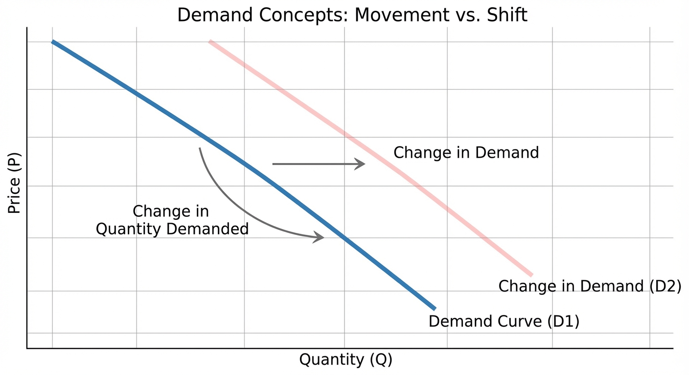
Changes in Demand vs. Changes in Quantity Demanded
This is perhaps the most critical distinction in Unit 2.
- Change in Quantity Demanded ($Q_d$):
- Cause: Caused only by a change in the current price of the good itself.
- Visual: Movement along the existing curve.
- Change in Demand:
- Cause: Caused by effective non-price determinants (Shifters).
- Visual: The entire curve shifts Left (decrease) or Right (increase).
Determinants of Demand (The Shifters)
Use the mnemonic TRIBE to remember what shifts the demand curve:
- Tastes and Preferences: Trends, studies, or seasons (e.g., studying says coffee is healthy $\rightarrow$ Demand shifts Right).
- Related Goods Prices:
- Substitutes: If Price of Pepsi $\uparrow$, Demand for Coke $\rightarrow$ (Direct relationship).
- Complements: If Price of Milk $\uparrow$, Demand for Cereal $\leftarrow$ (Inverse relationship).
- Income:
- Normal Goods: Income $\uparrow$, Demand $\rightarrow$ (e.g., steak, new cars).
- Inferior Goods: Income $\uparrow$, Demand $\leftarrow$ (e.g., ramen noodles, used cars).
- Buyers (Number of): More population = more demand.
- Expectations: If you expect prices to rise next week, you buy more today (Demand shifts Right).
The Mechanics of Supply
Supply refers to the different quantities of a good that sellers are willing and able to sell (produce) at different prices.
The Law of Supply
There is a direct relationship between price and quantity supplied.
- As Price ($P$) $\uparrow$, Quantity Supplied ($Q_s$) $\uparrow$
- As Price ($P$) $\downarrow$, Quantity Supplied ($Q_s$) $\downarrow$
Producers have a profit motive; higher prices encourage higher production. Graphically, the curve is upward-sloping.
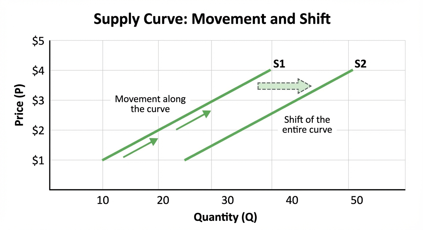
Determinants of Supply (The Shifters)
Just like demand, price changes only cause movement along the curve. To shift the curve, remember ROTTEN:
- Resource: Cost of inputs (labor, raw materials). If resource prices $\uparrow$, Supply $\leftarrow$ (becomes more expensive to produce).
- Other goods' prices: (Mainly relevant for substitutes in production).
- Technology: Better tech always shifts Supply $\rightarrow$.
- Taxes and Subsidies:
- Tax: Treated as a cost. Supply $\leftarrow$.
- Subsidy: Treated as a benefit/lowered cost. Supply $\rightarrow$.
- Expectations: If producers expect higher prices later, they may withhold supply now (Supply $\leftarrow$) to sell later.
- Number of Sellers: More firms entering the market shifts Supply $\rightarrow$.
Market Equilibrium
Equilibrium occurs where the Supply and Demand curves intersect ($Qd = Qs$). At this point, there is no tendency for price to change.
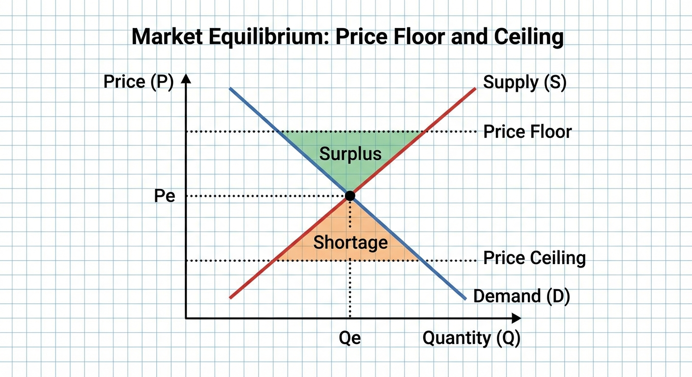
Disequilibrium
- Shortage: Occurs when Price is below equilibrium ($Qd > Qs$). Market forces will push the price up.
- Surplus: Occurs when Price is above equilibrium ($Qs > Qd$). Market forces will push the price down.
Double Shifts
When BOTH Demand and Supply shift simultaneously, one variable (Price or Quantity) will change predictably, but the other will be indeterminate (ambiguous) without specific numerical data.
| Shift Combination | Equilibrium Price ($P_e$) | Equilibrium Quantity ($Q_e$) |
|---|---|---|
| Demand $\uparrow$ / Supply $\uparrow$ | Indeterminate | Increase |
| Demand $\downarrow$ / Supply $\downarrow$ | Indeterminate | Decrease |
| Demand $\uparrow$ / Supply $\downarrow$ | Increase | Indeterminate |
| Demand $\downarrow$ / Supply $\uparrow$ | Decrease | Indeterminate |
Tip: Draw two separate graphs with different shift magnitudes to see which variable conflicts.
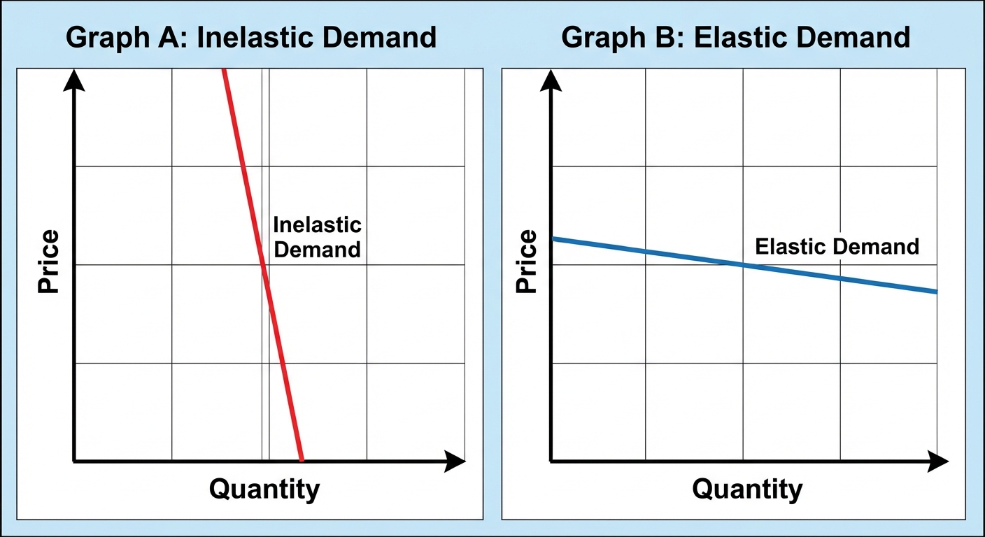
Elasticity
Elasticity measures sensitivity or responsiveness to price changes.
Price Elasticity of Demand (PED)
Measures how much quantity demanded responds to a change in price.
Note: In AP Microeconomics, we typically look at the absolute value of $E_d$.
| Coefficient | Classification | Interpretation | Shape of Curve |
|---|---|---|---|
| $ | E_d | > 1$ | Elastic |
| $ | E_d | < 1$ | Inelastic |
| $ | E_d | = 1$ | Unit Elastic |
The Total Revenue Test
Total Revenue ($TR$) = $Price \times Quantity$. The relationship between Price and TR determines elasticity.
- Inelastic Demand: Price and TR move in the same direction.
- If $P \uparrow$ and $TR \uparrow$, demand is Inelastic.
- Elastic Demand: Price and TR move in opposite directions.
- If $P \uparrow$ and $TR \downarrow$, demand is Elastic.
- Unit Elastic: Price changes, but TR remains unchanged (TR is maximized).
Other Elasticities
1. Cross-Price Elasticity of Demand (XED)
Measures how sensitive the demand for Good A is to the price of Good B.
- Positive (+): Goods are Substitutes (Price of Pepsi $\uparrow$, Q of Coke $\uparrow$).
- Negative (-): Goods are Complements (Price of Hot Dogs $\uparrow$, Q of Buns $\downarrow$).
2. Income Elasticity of Demand (YED)
Measures how sensitive demand is to a change in income.
- Positive (+): Normal Good.
- Negative (-): Inferior Good.
3. Price Elasticity of Supply (PES)
Measures how sensitive producers are to price changes. The primary determinant is Time.
- Short Run: Supply is Inelastic (hard to build new factories quickly).
- Long Run: Supply is Elastic (firms can adjust inputs/enter markets).
Common Mistakes & Pitfalls
"Change in Demand" vs. "Change in Quantity Demanded"
- Mistake: Saying "Price went up, so demand went down."
- Correction: "Price went up, so quantity demanded went down." (Movement along curve/slide). "Demand went down" implies the whole curve shifted left.
Confusion on Taxes/Subsidies
- Mistake: Shifting the Demand curve for a tax on producers.
- Correction: If the question says "Tax on Producers" or just "Excise Tax," shift Supply to the Left (vertical distance = tax amount).
Indeterminate Variables
- Mistake: Assuming both Price and Quantity change definitively during a double shift.
- Correction: Always remember one variable will be ambiguous. If Demand increases and Supply Increases, we know people are buying more ($Q$ increases), but price pressure is conflicting (Demand pulls P up, Supply pulls P down), so $P$ is indeterminate.
Elasticity Coefficient Signs
- Mistake: Ignoring the negative sign for XED or YED.
- Correction: For PED, we usually ignore the negative sign (absolute value). However, for Cross-Price and Income elasticity, the sign (+/-) is the most important part because it tells you the relationship (Substitute/Complement or Normal/Inferior).