Unit 7: Differential Equations - Formulation and Visualizations
Modeling with Differential Equations
In AP Calculus AB, a Differential Equation (DE) is simply an equation containing one or more derivatives of an unknown function. Before you solve these equations, you must learn how to translate real-world physical descriptions into mathematical statements involving derivatives.
Translating Words to Math
The key to modeling is recognizing that a "rate of change" corresponds to a derivative. If $y$ represents a quantity, $\frac{dy}{dt}$ represents how fast that quantity changes with respect to time.
Here represents a translation guide for common phrases found in AP Exam free-response questions:
| English Phrase | Mathematical Model |
|---|---|
| The rate of change of $y$ is proportional to $y$. | |
| The rate of change of $y$ is inversely proportional to $t$. | |
| The rate of change of $y$ is proportional to the difference between $y$ and an ambient temperature $A$ (Newton's Law of Cooling). | |
| The rate of change of $P$ is proportional to the product of $P$ and $10 - P$ (Logistic Growth). |
Key Variables:
- $k$: The constant of proportionality. If growth is increasing, $k > 0$. If obtaining decay, $k < 0$.
- $t$: The independent variable (usually time).
- $y$ (or $P$, $Q$, etc.): The dependent variable.
Example: Formulation
Scenario: A bacteria culture $B$ grows at a rate proportional to the square root of the amount of bacteria present.
Model:
Let $B(t)$ be the amount of bacteria at time $t$. The "rate" is $\frac{dB}{dt}$.
Verifying Solutions for Differential Equations
Unlike algebraic equations where the solution is a number (e.g., $x=5$), the solution to a differential equation is a function (e.g., $y = e^x$). You do not always need to solve a DE from scratch to verify if a function is a valid solution.
The Verification Process
To determine if a given function $y = f(x)$ is a solution to a differential equation:
- Differentiate the proposed solution to find $y'$ (and $y''$ if the DE is second-order).
- Substitute the function $y$ and its derivative $y'$ into the differential equation.
- Simplify both sides. If the Left Hand Side (LHS) equals the Right Hand Side (RHS), the function is a solution.
General vs. Particular Solutions
- General Solution: Contains an arbitrary constant $+C$ (e.g., $y = x^2 + C$). It represents a family of functions.
- Particular Solution: A specific function where $C$ has been solved using an Initial Condition (e.g., $y(0) = 3$).
Worked Example: Verification
Problem: Verify that $y = e^{-2x}$ is a solution to the differential equation $y' + 2y = 0$.
Step 1: Find the derivative.
Step 2: Substitute into the DE.
Step 3: Simplify.
Since the equation holds true, $y = e^{-2x}$ is indeed a solution.
Slope Fields
A Slope Field (or Direction Field) is a graphical tool used to visualize the general solution to a first-order differential equation. Since $\frac{dy}{dx}$ represents the slope of the tangent line, a slope field plots these slopes at various points on a coordinate grid.
Constructing a Slope Field
To sketch a slope field for $\frac{dy}{dx} = f(x,y)$:
- Create a grid of points (e.g., integer coordinates like $(0,0), (1,1)$, etc.).
- At each point $(x,y)$, calculate the value of the derivative $\frac{dy}{dx}$.
- Draw a short line segment at that point with the calculated slope.
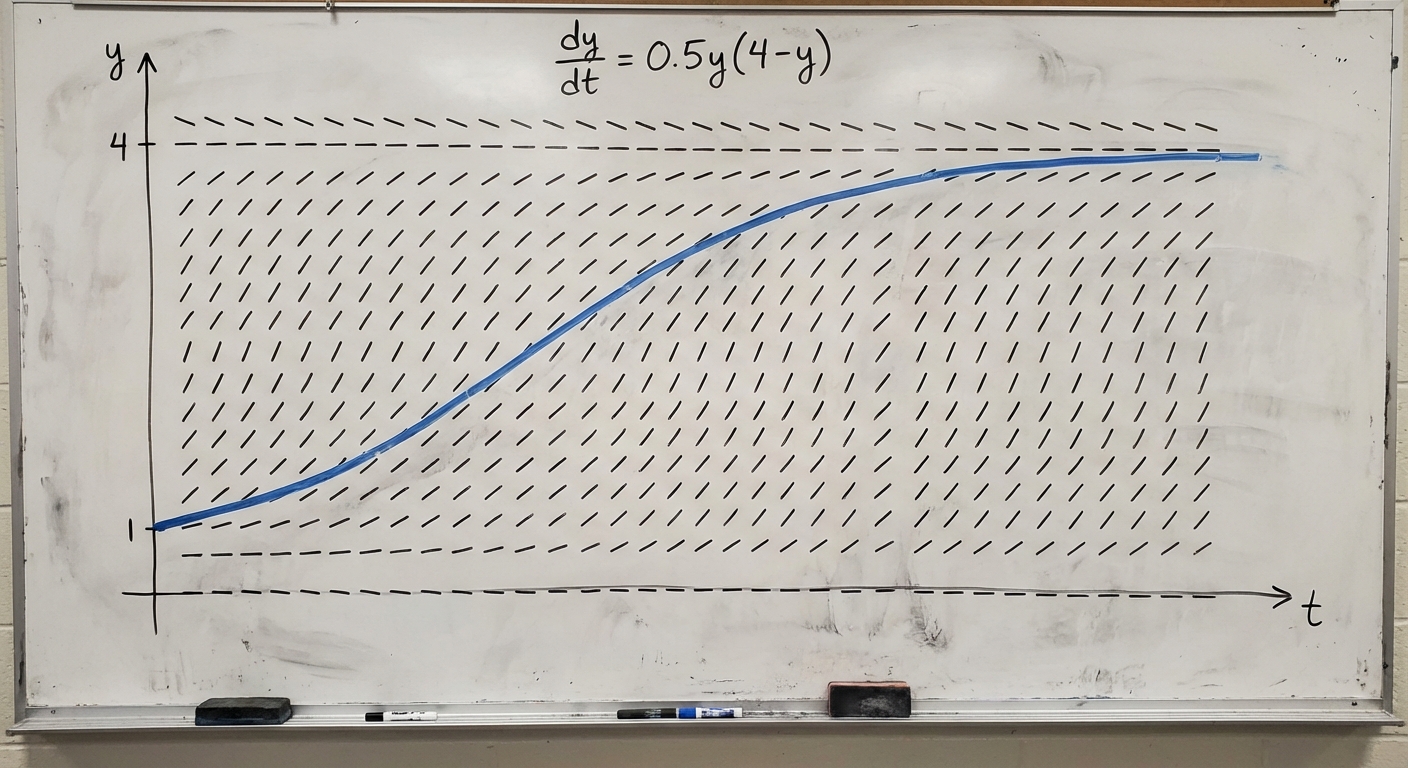
Interpreting Slope Fields (The "Flow")
Think of a slope field as a map of wind currents or water flow. A Solution Curve must follow the path of the segments. It must be differentiable (smooth) and cannot cross undefined regions.
- If you are given an initial condition $(x0, y0)$, start at that point and "follow the flow" to sketch the particular solution curve.
- Solution curves in a slope field never cross each other (due to the Uniqueness Theorem).
Patterns in Slope Fields
Recognizing patterns helps you match equations to graphs on multiple-choice questions:
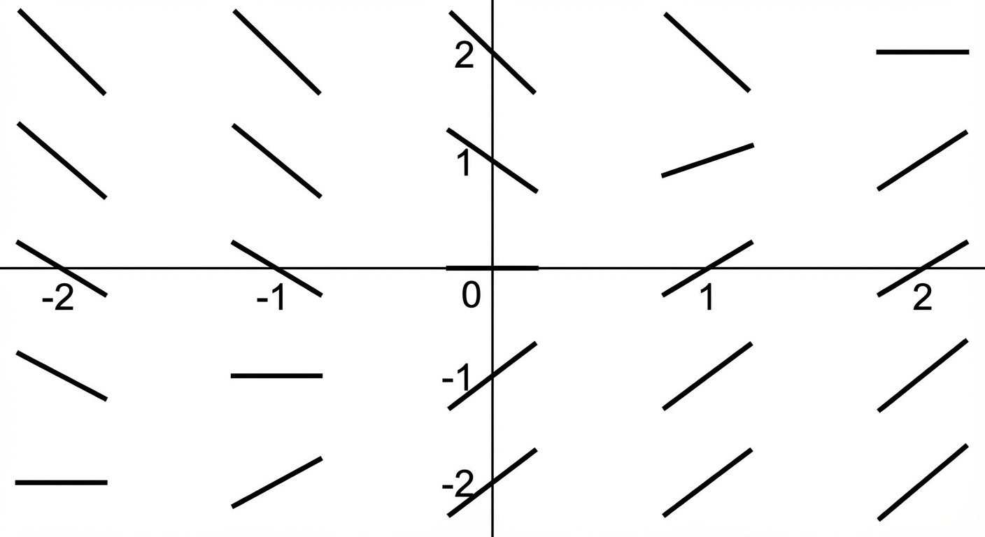
- Dependency on $x$ only: If $\frac{dy}{dx} = f(x)$ (e.g., $\frac{dy}{dx} = 2x$), the slopes are identical within every column. Vertical translation does not change the slope.
- Dependency on $y$ only: If $\frac{dy}{dx} = f(y)$ (e.g., $\frac{dy}{dx} = y - 1$), the slopes are identical within every row. Horizontal translation does not change the slope.
- Equilibrium Solutions: If for some constant $c$, $\frac{dy}{dx} = 0$ when $y=c$, look for a row of horizontal segments along the line $y=c$. This is a horizontal asymptote for the solution curves.
Common Mistakes & Pitfalls
- Slope Calculation Errors: Students often mentally swap $x$ and $y$ when plugging into the differential equation (e.g., for $\frac{dy}{dx} = y/x$, calculating $x/y$ instead). Tip: Write out a mini-table of coordinate pairs before drawing.
- Undefined Slopes: If the derivative is undefined (e.g., division by zero), do not draw a vertical line segment. Leave that point blank on the slope field grid.
- Ignoring Solution Domain: When sketching a solution curve through a slope field, you cannot cross vertical asymptotes. Solution curves are continuous functions defined on an interval.