AP Precalculus Study Guide: Dimensions of Modeling & Transformations
Function Modeling and Transformations
This guide covers the essential mechanics of manipulating functions and using them to model real-world data, corresponding to key topics in Unit 1 of the AP Precalculus curriculum.
Transformations of Functions
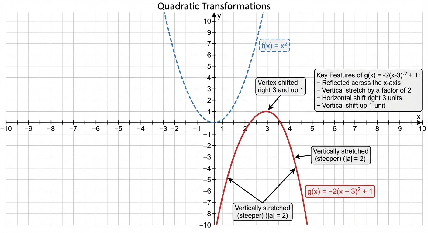
Understanding how to effectively alter a parent function is foundational to precalculus. These transformations allow you to reposition and reshape graphs to fit specific criteria.
The General Transformation Formula
Given a function $f(x)$, the transformed function $g(x)$ can be written as:
Where each parameter controls a specific geometric change:
$a$ (Vertical Operations):
- $|a| > 1$: Vertical stretch by a factor of $|a|$.
- $0 < |a| < 1$: Vertical compression (shrink) by a factor of $|a|$.
- $a < 0$: Reflection over the x-axis.
$b$ (Horizontal Operations):
- $|b| > 1$: Horizontal compression by a factor of $\frac{1}{|b|}$.
- $0 < |b| < 1$: Horizontal stretch by a factor of $\frac{1}{|b|}$.
- $b < 0$: Reflection over the y-axis.
- Note: Horizontal changes happen inside the function grouping and affect the input variable $x$.
$h$ (Horizontal Shift):
- Shift right if $(x - h)$ where $h > 0$.
- Shift left if $(x + h)$ implies $h < 0$.
$k$ (Vertical Shift):
- Shift up if $k > 0$.
- Shift down if $k < 0$.
Order of Transformations
The standard order derived from the formula above is:
- Horizontal Shift ($h$)
- Horizontal Stretch/Shrink/Reflection ($b$)
- Vertical Stretch/Shrink/Reflection ($a$)
- Vertical Shift ($k$)
However, if the input is written as $(bx - c)$, you must factor out the $b$ first to identify the true phase shift: $b(x - \frac{c}{b})$.
Mnemonic: "Inside is Inverse"
When dealing with transformations inside the parentheses (horizontal $b$ and $h$), the action is the intuitive "inverse" of what you see.
- See $x - 3$? Go Right (add 3 to x).
- See $2x$? Divide x-values by 2 (shrink).
Use of Regression and Residual Analysis
In AP Precalculus, you are not expected to calculate least-squares regression lines by hand. Instead, you must allow technology to generate a model and then analyze how well that model fits the data.
Linear and Polynomial Regression
regression involves fitting a function curve to a set of data points to minimize the distance between the data and the curve.
- Correlation Coefficient ($r$): Measures the strength and direction of a linear relationship. $-1 \leq r \leq 1$. The closer $|r|$ is to 1, the stronger the linear relationship.
- Coefficient of Determination ($r^2$): Represents the proportion of variation in the dependent variable explained by the independent variable.
Residual Analysis
The residual is the vertical distance between the actual data point and the predicted model value:
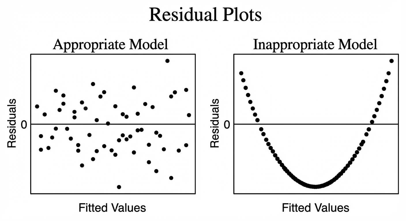
To determine if a function model is appropriate, we examine a Residual Plot (x-axis vs. Residuals).
- Random Scatter: If the residual plot shows a random cloud of points with no discernible shape, the model chosen (e.g., linear) is appropriate.
- Patterned Shape: If the residual plot shows a clear pattern (like a U-shape or a curve), the model chosen is inappropriate. Even if the $r$-value is high, a pattern in the residuals implies there is underlying non-linear behavior that the current model failed to capture.
Function Model Selection and Construction
When given a data set without technology, you must determine if it behaves linearly, quadratically, or otherwise.
Analyzing Rates of Change
Linear Models:
- The First Differences of output values are constant (for equally spaced inputs).
- The rate of change is constant.
Quadratic Models:
- The First Differences are not constant (they change linearly).
- The Second Differences (the difference of the differences) are constant and non-zero.
Concavity:
- Concave Up: Rate of change is increasing.
- Concave Down: Rate of change is decreasing.
Piecewise-Defined Functions
Piecewise functions describe real-world scenarios where rules change based on the input level—such as tax brackets, shipping costs, or tiered data plans.
Concept & Notation
A piecewise function is defined by different formulas over distinct intervals of the domain.
f(x) = \begin{cases}
2x + 1 & \text{if } x < 0 \
x^2 & \text{if } x \geq 0
\end{cases}
Continuity at the Break
To determine if the function is continuous at the "break point" (e.g., $x=c$):
- Evaluate the first rule at $x=c$.
- Evaluate the second rule at $x=c$.
- If the values match, the function is continuous (connected). If not, there is a jump discontinuity.
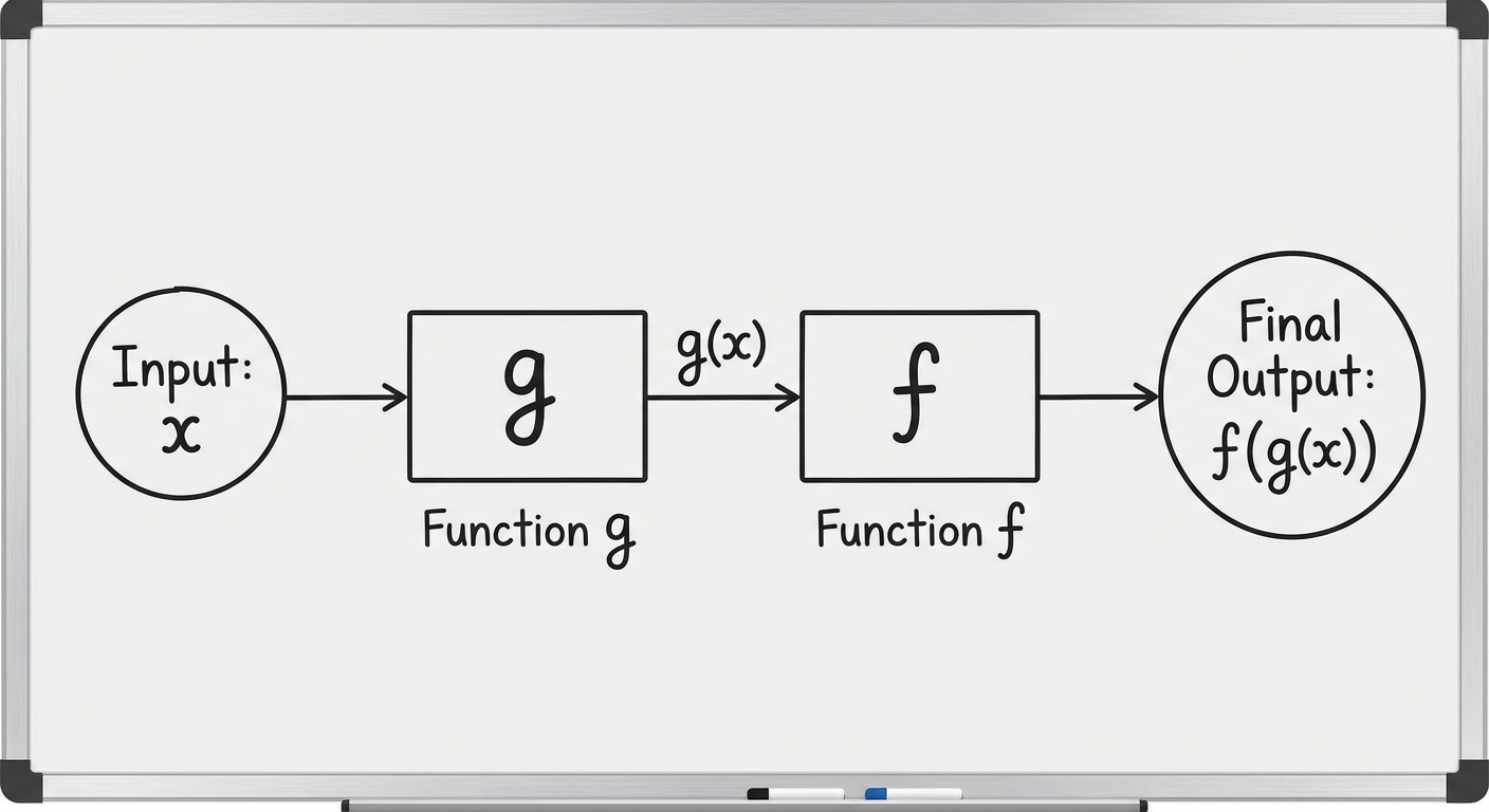
Composition of Functions
Composition involves using the output of one function as the input for another. This is denoted as $(f \circ g)(x) = f(g(x))$.
The Domain constraint
The domain of $f(g(x))$ consists of all $x$ in the domain of $g$ such that $g(x)$ is in the domain of $f$.
Example:
Let $f(x) = \sqrt{x}$ and $g(x) = x - 4$.
- $f(g(x)) = \sqrt{x - 4}$.
- Domain of $g$: $(-\infty, \infty)$.
- Domain of $f$: $[0, \infty)$.
- Therefore, we explicitly need the output of $g$ ($x-4$) to be $\geq 0$.
- Final Domain: $x \geq 4$, or $[4, \infty)$.
Common Mistakes & Pitfalls
The Factor-Out Failure (Horizontal Shifts):
- Mistake: Thinking $y = f(2x - 6)$ is a shift right by 6.
- Correction: You must factor out the 2 first: $y = f(2(x - 3))$. The shift is right by 3.
Order of Operations (Transformations):
- Mistake: Evaluating vertical shifts before stretches/reflections.
- Correction: Always multiply/reflect before you add/subtract (PEMDAS applies to function mapping too).
Residual Misinterpretation:
- Mistake: Thinking a pattern in the residual plot is "good" because it looks organized.
- Correction: In residuals, chaos is good. Patterns mean the model missed something (e.g., trying to fit a line to a curve).
Composition Domains:
- Mistake: Finding the domain after simplifying the final equation only.
- Correction: You must consider the restrictions of the inner function $g(x)$ before simplification. For example, in $f(g(x))$ where $g(x) = \sqrt{x}$ and $f(x) = x^2$, the composite simplifies to $x$, but the domain is only $x \ge 0$ because $g(x)$ cannot process negatives.