Mastering Differential Equations: Modeling, Visualization, and Approximation
Modeling Situations with Differential Equations
In AP Calculus BC, a Differential Equation (DE) is simply an equation containing one or more derivatives of an unknown function. Before solving them mathematically, you must be able to translate verbal descriptions of physical phenomena into mathematical equations.
Key Keywords & Translations
The difficulty often lies in translating the sentence "The rate of change of $y$" into the symbol $\frac{dy}{dt}$. Below is a translation guide for common modeling scenarios:
| Verbal Description | Mathematical Model |
|---|---|
| Rate of change of $y$ is proportional to $y$. | |
| Rate of change of $y$ is inversely proportional to $x$. | |
| Rate of change of $y$ is proportional to the square of $y$. | |
| Rate of change of $y$ is proportional to the difference between $y$ and a constant $A$. |
Note: $k$ is the constant of proportionality. If the problem states the quantity is increasing, $k > 0$. If decreasing, $k < 0$ (or the equation is written with a negative sign, e.g., $-ky$).
Example: Newton's Law of Cooling
Scenario: The rate at which an object cools is proportional to the difference between the object's temperature ($T$) and the surrounding room temperature ($T_s$).
Model:
If the object is hotter than the room ($T > T_s$), the temperature must decrease, implying the derivative must be negative. Therefore, in this specific context, $k$ would be a negative constant.
Verifying Solutions for Differential Equations
You effectively "solve" a differential equation when you find a function $y = f(x)$ that makes the equation true. Sometimes, AP questions ask you to verify a solution rather than derive it from scratch.
The Verification Process
To check if a specific function is a solution to a given differential equation:
- Identify the proposed solution $y$ and the differential equation.
- Differentiate the proposed solution to find $y'$, $y''$, etc., as needed by the DE.
- Substitute $y$ and its derivatives into the DE.
- Simplify both sides. If LHS = RHS, the solution is valid.
Worked Practice
Problem: Verify that $y = e^{-2x}$ is a solution to the differential equation $y' + 2y = 0$.
Step 1: Differentiate the proposed solution.
Step 2: Substitute into the DE.
Substitute $y$ and $y'$ into the left side of $y' + 2y = 0$:
Step 3: Simplify.
Since $0 = 0$, the function satisfies the equation.
Sketching and Interpreting Slope Fields
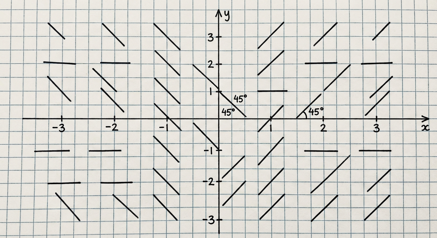
A Slope Field (or Direction Field) is a graphical tool used to visualize the general shape of solutions to a differential equation without algebraically solving it. It represents the value of the derivative $\frac{dy}{dx}$ (the slope of the tangent line) at various points $(x,y)$ on a coordinate plane.
How to Sketch a Slope Field
You will often be given a grid of points (e.g., integer coordinates from -2 to 2) and asked to draw the field.
- Select a point $(x, y)$ indicated on the grid.
- Calculate the slope value at that point using the given DE: $m = \frac{dy}{dx}$.
- Draw a short line segment through that point with slope $m$.
- Slope $0$: Horizontal line (---)
- Slope $1$: Diagonal up ($45^\circ$)
- Slope $-1$: Diagonal down
- Slope $\text{undefined}$: Vertical line (usually indicated by no line or a vertical tick)
Analyzing Patterns (The "Cheat Codes")
When trying to match an equation to a graph on a multiple-choice question, look for these structural cues:
- Functions of $x$ only (e.g., $\frac{dy}{dx} = x$): Slopes are the same within every vertical column. (Consider $(1,0), (1,1), (1,2)$—if $x$ doesn't change, the slope doesn't change).
- Functions of $y$ only (e.g., $\frac{dy}{dx} = y$): Slopes are the same within every horizontal row.
- Equilibrium Solutions: Look where the slope is $0$. If $\frac{dy}{dx} = y - 2$, the slope is zero anywhere $y=2$. You should see horizontal segments all along the line $y=2$.
Euler's Method (AP Calculus BC Only)
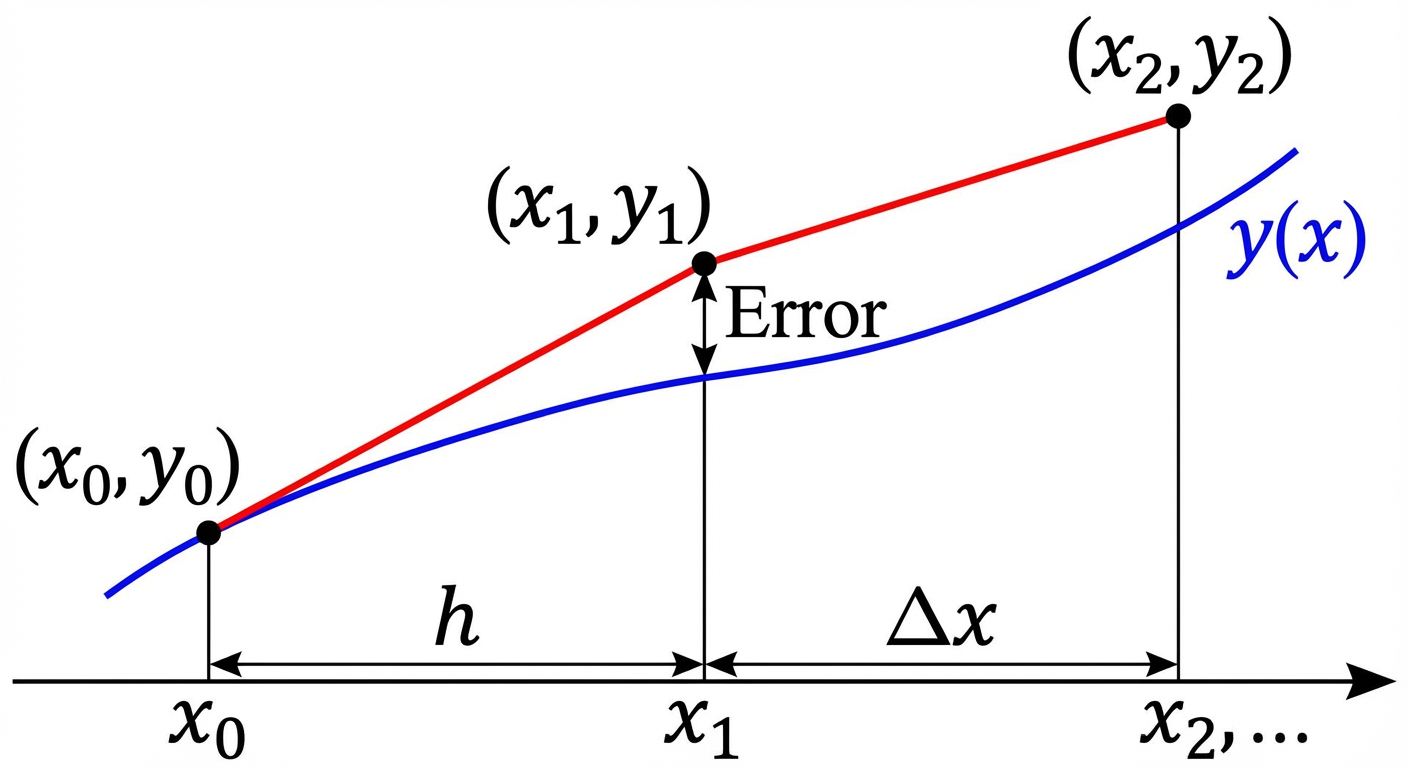
Euler's Method is a numerical approach used to approximate the particular solution of a differential equation $y' = f(x,y)$ passing through a given initial condition $(x0, y0)$. It essentially links together a series of short tangent lines to "step" from a known point to an approximate future point.
The Algorithm
Given a step size $\Delta x$ (sometimes called $h$):
Or, more formally:
Worked Example
Problem: Given $\frac{dy}{dx} = x + y$ and $y(0) = 1$, approximate $y(0.2)$ using two equal steps of size $\Delta x = 0.1$.
Step 1: Identify parameters.
- Initial point $(x0, y0) = (0, 1)$
- Step size $\Delta x = 0.1$
- Goal: Find $y$ when $x = 0.2$
Step 2: First Iteration (finding $y_1$ at $x=0.1$)
- Calculate slope at $(0,1)$: $\frac{dy}{dx} = 0 + 1 = 1$
- Calculate new $y$: $y_1 = 1 + (1)(0.1) = 1.1$
- New point: $(0.1, 1.1)$
Step 3: Second Iteration (finding $y_2$ at $x=0.2$)
- Calculate slope at $(0.1, 1.1)$: $\frac{dy}{dx} = 0.1 + 1.1 = 1.2$
- Calculate new $y$: $y_2 = 1.1 + (1.2)(0.1) = 1.1 + 0.12 = 1.22$
- Answer: $y(0.2) \approx 1.22$
Common Mistakes & Pitfalls
1. Arithmetic Errors in Euler's Method
This is the #1 killer of points on BC FRQs. Since Euler's method is recursive (the next answer depends on the previous one), a single calculation error at Step 1 ruins the entire problem. Tip: Organize your work in a 3-column table: Point $(x,y)$, Slope $\frac{dy}{dx}$, and New $y$.
2. Confusing Variables in Slope Fields
Students often calculate slopes based on $x$ when the equation depends on $y$ (or vice versa).
- Check: If $\frac{dy}{dx} = 2y$, the slope at $(3, 1)$ depends only on $y=1$, so the slope is 2. Do not plug in $x=3$.
3. Concavity and Euler's Approximation
Remember the relationship between concavity and over/under estimation:
- If the solution curve is concave up, the tangent lines lie below the curve, so Euler's method produces an underestimation.
- If the solution curve is concave down, tangent lines lie above, producing an overestimation.
4. Forgetting Signs in Modeling
When modeling "rate of cooling" or "rate of decay," the concept implies a decrease, but the derivative $\frac{dy}{dt}$ must be negative. Ensure your constant $k$ or the sign in front of the equation reflects this ($ -k(y-A)$ or $k$ where $k<0$).