AP Calculus AB Unit 4: Linearization (Local Linearity, Differentials) and L'Hôpital's Rule
Local Linearity and Linearization
What “local linearity” means
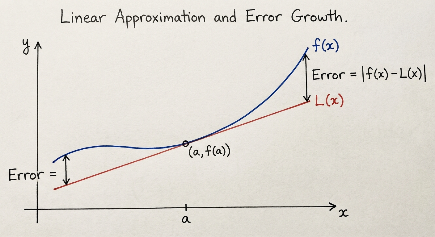
Local linearity is the idea that if a function is differentiable at a point, then when you zoom in close enough to that point, the graph becomes almost indistinguishable from a straight line. That straight line is the tangent line. This does not mean the function is actually linear; it means that near a specific input value, a differentiable function behaves approximately like its tangent line.
The reason this works is that the derivative at a point captures the instantaneous rate of change there, and the tangent line is the unique line that matches both the function’s value and the function’s slope at that point. So near the point of tangency, the tangent line is the best linear “stand-in” for the curve.
Why it matters (especially in applications)
In contextual problems, you often want to estimate a quantity when an exact computation is hard (like evaluating a complicated function by hand) or when you only have measurements with small errors and want to understand how those errors affect the output. Local linearity gives you a powerful tool: you can approximate complicated behavior with a simple linear model as long as you stay close to the point of tangency.
This shows up everywhere: physics (small changes in position or velocity), economics (marginal cost or marginal revenue), biology (small changes in concentration), and measurement error analysis.
The tangent line (linearization) formula, with a quick derivation
Linearization is the process of finding the equation of the tangent line at a chosen point and using it to estimate values of the function nearby.
Start from the point-slope form of a line:
y-y_1=m(x-x_1)
To approximate %%LATEX1%% near %%LATEX2%%:
- The point of tangency is %%LATEX3%%, so %%LATEX4%% and y_1=f(a).
- The slope is the derivative at that point, so m=f'(a).
Substituting into point-slope form gives the tangent line equation:
y-f(a)=f'(a)(x-a)
Solving for y gives the standard linearization (also called the standard linear approximation or tangent line approximation):
L(x)=f(a)+f'(a)(x-a)
When %%LATEX10%% is close to %%LATEX11%%, you use:
f(x)\approx L(x)
Interpretation: %%LATEX13%% is the baseline value, and %%LATEX14%% adjusts that baseline using the slope and how far you move from a.
Equivalent “small change” viewpoint (differentials)
Another way to express local linearity is to approximate a small change in output using the derivative.
Let:
\Delta x=x-a
Then the actual change in output is:
\Delta y=f(a+\Delta x)-f(a)
Local linearity says that for small \Delta x,
\Delta y\approx f'(a)\Delta x
You will also see differentials written as:
dy=f'(x)dx
When evaluating near %%LATEX21%%, you often take %%LATEX22%% and estimate:
\Delta y\approx dy=f'(a)\Delta x
Conceptually, this is the same idea as linearization, just framed as “small input change produces approximately slope times input change.”
Notation reference (common equivalent language)
| Idea | Common notation | Meaning |
|---|---|---|
| Linearization at a | L(x)=f(a)+f'(a)(x-a) | Best linear model near x=a |
| Tangent line at a | y-f(a)=f'(a)(x-a) | Same line, different form |
| Small-change approximation | \Delta y\approx f'(a)\Delta x | Output change from small input change |
| Differential form | dy=f'(a)dx | Linear estimate of change |
How to use linearization effectively
A good approximation depends as much on choosing the right point as it does on computing correctly.
- Choose a nearby “friendly” input %%LATEX31%% where you can compute %%LATEX32%% easily (for roots, pick a perfect square/cube nearby; for trig, pick a special angle).
- Compute the derivative %%LATEX33%% and evaluate %%LATEX34%%.
- Build the linearization L(x)=f(a)+f'(a)(x-a).
- Plug the target value %%LATEX36%% into %%LATEX37%%, making sure %%LATEX38%% is close to %%LATEX39%%.
The most common failure mode is using a point a that is not close enough; then the curve’s nonlinearity matters and the tangent line stops being accurate.
Worked Example 1: Approximating a square root
Approximate \sqrt{10} without a calculator.
Choose %%LATEX42%% and a nearby easy point %%LATEX43%%.
Derivative:
f'(x)=\frac{1}{2\sqrt{x}}
Evaluate at 9:
f(9)=3
f'(9)=\frac{1}{6}
Linearization at 9:
L(x)=3+\frac{1}{6}(x-9)
Evaluate at x=10:
L(10)=3+\frac{1}{6}(1)=3.166666\ldots
So:
\sqrt{10}\approx 3.1667
A quick reasonableness check: %%LATEX53%% should be a bit bigger than %%LATEX54%% and not close to 4, so this fits.
Worked Example 2: Approximating a root (another nearby-square setup)
Use linearization to approximate \sqrt{4.1}.
Choose %%LATEX57%% and %%LATEX58%% since \sqrt{4}=2.
Derivative:
f'(x)=\frac{1}{2\sqrt{x}}
Evaluate at 4:
f(4)=2
f'(4)=\frac{1}{4}=0.25
Linearization:
L(x)=2+0.25(x-4)
Approximate:
L(4.1)=2+0.25(0.1)=2.025
Note: the actual value of %%LATEX66%% is approximately %%LATEX67%%, so this approximation is accurate to three decimal places.
Worked Example 3: Estimating change in context (differentials / error)
Suppose the radius %%LATEX68%% of a sphere is measured as %%LATEX69%% cm, but the measurement could be off by 0.1 cm. Estimate the resulting possible error in the volume.
Volume:
V=\frac{4}{3}\pi r^3
Treat the measurement error as a small change \Delta r\approx \pm 0.1 and use:
\Delta V\approx \frac{dV}{dr}\Delta r
Derivative:
\frac{dV}{dr}=4\pi r^2
At r=10:
\frac{dV}{dr}=4\pi (10)^2=400\pi
Estimated error:
\Delta V\approx 400\pi(\pm 0.1)=\pm 40\pi
So a radius measurement error of about %%LATEX78%% cm leads to a volume error of about %%LATEX79%% cubic centimeters. Interpretation: volume is very sensitive to radius because it scales like r^3.
Overestimates vs underestimates (using concavity)
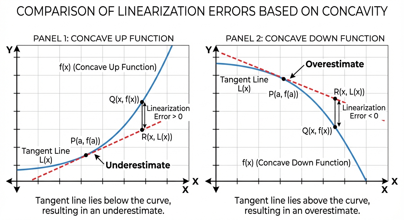
A subtle but important point is that the tangent line approximation can systematically overestimate or underestimate depending on the function’s concavity near a.
- If %%LATEX82%% is concave up near %%LATEX83%% (so %%LATEX84%% nearby), the graph lies above its tangent lines, so for %%LATEX85%% near a:
L(x)\le f(x)
This means the linearization is an underestimate.
- If %%LATEX88%% is concave down near %%LATEX89%% (so %%LATEX90%% nearby), the graph lies below its tangent lines, so for %%LATEX91%% near a:
L(x)\ge f(x)
This means the linearization is an overestimate.
| Concavity | Significance | Tangent line position | Result |
|---|---|---|---|
| Concave Up | f''(x)>0 | Below the curve | Underestimate L(x) |
| Concave Down | f''(x) |
Mnemonic: think of a cup (concave up). If you lay a ruler (tangent line) under the cup, it sits below it.
What goes wrong (common pitfalls)
Local linearity is powerful, but it has boundaries.
If you do not stay local (your target %%LATEX98%% is not close to %%LATEX99%%), the error can be large because the curve bends away from the tangent line. A second common mistake is mixing up %%LATEX100%% and %%LATEX101%%: in %%LATEX102%%, the “change” is %%LATEX103%%, not %%LATEX104%%. In contextual problems, forgetting units is another trap: derivatives and differentials carry units (for example, %%LATEX105%% has units of volume per length), and unit-checking often reveals setup mistakes.
Finally, don’t confuse concavity with increasing or decreasing behavior. Whether the approximation overestimates or underestimates is determined by %%LATEX106%%, not by the sign of %%LATEX107%%.
Exam Focus
Typical question patterns include: using linearization at %%LATEX108%% to approximate %%LATEX109%% where %%LATEX110%% is close to %%LATEX111%%; estimating the change in a quantity using \Delta y\approx f'(a)\Delta x in a real-world context; and determining whether the linear approximation is an overestimate or underestimate using concavity.
Common mistakes include: choosing a point %%LATEX113%% that is not close to the target value; computing %%LATEX114%% correctly but then forgetting to evaluate the derivative at %%LATEX115%% when building the approximation; mixing up %%LATEX116%% with %%LATEX117%%; and deciding over/underestimate from the sign of %%LATEX118%% instead of the sign of f''(a).
L'Hôpital's Rule
Where L'Hôpital’s Rule fits (and an AP Calculus AB honesty note)
When evaluating limits, you often substitute the approaching value. If you get a normal real number, you are done. But sometimes substitution produces an indeterminate form, meaning the expression does not have a determined limit just from the visible algebra.
L'Hôpital’s Rule is a technique for evaluating limits that result in the indeterminate forms:
\frac{0}{0}
or
\frac{\infty}{\infty}
Important curriculum note: L'Hôpital’s Rule is required in AP Calculus BC. It is commonly taught as enrichment in AB, but it is not consistently an assessed AB exam skill. Even when it is not tested directly, it strengthens your understanding of limits and connects differentiation to limit behavior.
What an “indeterminate form” really means
An indeterminate form does not mean “the limit does not exist.” It means “this form alone does not tell you what the limit is.”
For example, as %%LATEX122%% approaches %%LATEX123%%, both of the following produce the substitution form \frac{0}{0}, but the limits differ:
\frac{x}{x}\to 1
\frac{x^2}{x}\to 0
So you need additional analysis.
Indeterminate forms L'Hôpital applies to (and the ones you must rewrite)
L'Hôpital’s Rule can only be applied directly when substitution gives one of these two forms:
\frac{0}{0}
\frac{\pm \infty}{\pm \infty}
Other indeterminate forms require algebraic rewriting first, such as:
0\cdot\infty
\infty-\infty
0^0
1^\infty
\infty^0
Statement of L'Hôpital's Rule (usable version)
Suppose %%LATEX134%% and %%LATEX135%% are differentiable on an interval around %%LATEX136%% (except possibly at %%LATEX137%%), and %%LATEX138%% near %%LATEX139%%. If:
\lim_{x\to a}\frac{f(x)}{g(x)}
produces the indeterminate form %%LATEX141%% or %%LATEX142%%, then (under appropriate conditions):
\lim_{x\to a}\frac{f(x)}{g(x)}=\lim_{x\to a}\frac{f'(x)}{g'(x)}
provided the limit on the right exists (or diverges to %%LATEX144%% or %%LATEX145%%). The same idea applies to one-sided limits and limits as x\to\infty.
Why the rule makes sense (intuition)
At a high level, L'Hôpital’s Rule compares how fast the numerator and denominator approach 0 (or grow without bound). Since derivatives measure instantaneous rates of change, taking derivatives of numerator and denominator is a way of comparing their dominant behavior near the limiting point.
You can connect this to local linearity: near x=a, differentiable functions are approximately linear, so you can think roughly:
f(x)\approx f'(a)(x-a)
g(x)\approx g'(a)(x-a)
If both go to 0, then the ratio behaves like:
\frac{f(x)}{g(x)}\approx \frac{f'(a)(x-a)}{g'(a)(x-a)}=\frac{f'(a)}{g'(a)}
This is intuition rather than a proof, but it explains why derivatives show up.
How to apply L'Hôpital’s Rule (a reliable process)
- Check for an indeterminate form by substitution. If you do not have %%LATEX153%% or %%LATEX154%%, do not apply the rule.
- Differentiate numerator and denominator separately. Do not use the quotient rule; you are not differentiating the quotient as a function, you are forming a new fraction.
- Re-evaluate the new limit by substitution or simplification.
- Repeat only if the result is still %%LATEX155%% or %%LATEX156%%. Multiple applications are allowed.
A key habit is to pause after each application and re-check the form. Many mistakes come from applying the rule automatically without confirming it still applies.
Important exam procedure (especially for free-response)
On AP-style free-response, you must show the conditions clearly. You should not write that a limit “equals” \frac{0}{0}. Instead, explicitly evaluate the numerator and denominator limits separately, then invoke the rule.
A correct work-flow sentence looks like this:
Since:
\lim_{x\to c} f(x)=0
and:
\lim_{x\to c} g(x)=0
by L'Hôpital’s Rule:
\lim_{x\to c}\frac{f(x)}{g(x)}=\lim_{x\to c}\frac{f'(x)}{g'(x)}
Worked Example 1: A classic \frac{0}{0} limit
Evaluate:
\lim_{x\to 0}\frac{\sin x}{x}
Substitution gives \frac{0}{0}, so apply L'Hôpital:
\lim_{x\to 0}\frac{\sin x}{x}=\lim_{x\to 0}\frac{\cos x}{1}
Now substitute:
\cos 0=1
So the limit is:
1
Note: In AP Calculus AB, this limit is typically established using the Squeeze Theorem or known special limit results, not necessarily via L'Hôpital’s Rule, but L'Hôpital confirms the same result.
Worked Example 2: The standard chain-rule case
Evaluate:
\lim_{x\to 0}\frac{\sin(3x)}{x}
Substitution gives \frac{0}{0}.
Differentiate top and bottom separately:
\frac{d}{dx}(\sin(3x))=3\cos(3x)
\frac{d}{dx}(x)=1
So:
\lim_{x\to 0}\frac{\sin(3x)}{x}=\lim_{x\to 0}\frac{3\cos(3x)}{1}
Evaluate:
3\cos(0)=3
Worked Example 3: An \frac{\infty}{\infty} limit (comparing growth)
Evaluate:
\lim_{x\to\infty}\frac{3x^2+5}{7x^2-4x}
Both numerator and denominator go to \infty, so apply L'Hôpital:
\lim_{x\to\infty}\frac{3x^2+5}{7x^2-4x}=\lim_{x\to\infty}\frac{6x}{14x-4}
This is still \frac{\infty}{\infty}, so apply again:
\lim_{x\to\infty}\frac{6x}{14x-4}=\lim_{x\to\infty}\frac{6}{14}
So the limit is:
\frac{3}{7}
This matches what you might get by dividing by x^2, but L'Hôpital is another systematic approach.
Worked Example 4: The “exponential dominates polynomial” case
Evaluate:
\lim_{x\to\infty}\frac{2x^2}{e^x}
This is \frac{\infty}{\infty}. Apply L'Hôpital:
\lim_{x\to\infty}\frac{2x^2}{e^x}=\lim_{x\to\infty}\frac{4x}{e^x}
Still \frac{\infty}{\infty}, so apply again:
\lim_{x\to\infty}\frac{4x}{e^x}=\lim_{x\to\infty}\frac{4}{e^x}
Now the numerator approaches %%LATEX186%% and the denominator approaches %%LATEX187%%, so the limit is:
0
Handling other indeterminate forms (rewrite first)
L'Hôpital’s Rule only applies directly to ratios giving %%LATEX189%% or %%LATEX190%%. If you see a different indeterminate form, rewrite it into one of those forms first.
Rewrite type A: Product 0\cdot\infty to a quotient
Evaluate:
\lim_{x\to 0^+} x\ln x
As %%LATEX193%%, you have %%LATEX194%%, which is indeterminate. Rewrite:
x\ln x=\frac{\ln x}{1/x}
Now as %%LATEX196%%, the form is %%LATEX197%%, so apply L'Hôpital:
\lim_{x\to 0^+}\frac{\ln x}{1/x}=\lim_{x\to 0^+}\frac{1/x}{-1/x^2}
Simplify:
\frac{1/x}{-1/x^2}=-x
So:
\lim_{x\to 0^+} -x=0
Therefore:
\lim_{x\to 0^+} x\ln x=0
A common error is to think “%%LATEX202%% goes to negative infinity so the product must go to negative infinity.” The key is that %%LATEX203%% goes to 0 fast enough to dominate.
Rewrite type B: Power forms using logarithms
Evaluate:
\lim_{x\to\infty}\left(1+\frac{1}{x}\right)^x
This is the indeterminate form 1^\infty. Let:
y=\left(1+\frac{1}{x}\right)^x
Take natural log:
\ln y=x\ln\left(1+\frac{1}{x}\right)
Now consider:
\lim_{x\to\infty} x\ln\left(1+\frac{1}{x}\right)
This is \infty\cdot 0, so rewrite as a quotient:
x\ln\left(1+\frac{1}{x}\right)=\frac{\ln\left(1+\frac{1}{x}\right)}{1/x}
Now it is %%LATEX212%% as %%LATEX213%%, so apply L'Hôpital.
Differentiate numerator:
\frac{d}{dx}\left[\ln\left(1+\frac{1}{x}\right)\right]=\frac{-1/x^2}{1+1/x}
Differentiate denominator:
\frac{d}{dx}\left[\frac{1}{x}\right]=-\frac{1}{x^2}
So the limit becomes:
\lim_{x\to\infty}\frac{\frac{-1/x^2}{1+1/x}}{-1/x^2}
Cancel the common factor to get:
\lim_{x\to\infty}\frac{1}{1+1/x}
As %%LATEX218%%, %%LATEX219%%, so:
\lim_{x\to\infty} \ln y=1
Exponentiate to return to y:
\lim_{x\to\infty} y=e
Thus:
\lim_{x\to\infty}\left(1+\frac{1}{x}\right)^x=e
This approach is more advanced than typical AB exam expectations, but it shows the general strategy for exponential indeterminate forms.
What goes wrong (common pitfalls)
A major pitfall is applying the rule when the form is not indeterminate. For example, if substitution gives \frac{2}{0}, that is not indeterminate; it signals vertical asymptote behavior, and L'Hôpital is not the right first move.
Another frequent issue is the quotient rule trap: differentiating the entire fraction as a function using the quotient rule instead of differentiating numerator and denominator independently. Also, after each application, you must re-check the form; sometimes you need to simplify first, sometimes one application is enough, and sometimes multiple applications are required.
Finally, be careful with notation on free-response: never write a limit “equals” %%LATEX225%%. Instead, state that the numerator and denominator limits are individually %%LATEX226%% (or both infinite), then invoke the rule.
Exam Focus
Typical question patterns include evaluating limits where direct substitution yields %%LATEX227%% or %%LATEX228%%; showing a limit diverges by producing %%LATEX229%% or %%LATEX230%% after applying the rule; and evaluating an indeterminate form after algebraic manipulation (especially rewriting products as quotients).
Common mistakes include: using the quotient rule instead of differentiating numerator and denominator separately; forgetting to verify the form is %%LATEX231%% or %%LATEX232%% before applying L'Hôpital; applying L'Hôpital to products or differences without rewriting into a single quotient first; stopping after one application even though the result is still indeterminate; and writing incorrect FRQ notation like equating a limit to \frac{0}{0}.
Summary of Common Mistakes (Quick Checklist)
- The Quotient Rule Trap (L'Hôpital): L'Hôpital requires %%LATEX234%%, not the quotient rule derivative of %%LATEX235%%.
- Forgetting to Check Conditions (L'Hôpital): If substitution does not give %%LATEX236%% or %%LATEX237%%, do not apply the rule.
- Concavity Confusion (Linearization): Over/underestimation is determined by %%LATEX238%%, not by whether %%LATEX239%% is increasing or decreasing.
- Notation Errors (FRQ limits): Do not write that a limit equals \frac{0}{0}; state the numerator and denominator limits separately, then apply the rule.
Exam Focus
Use this as a final pre-test scan. If you can explain why each item is a mistake and what the correct method is, you are much less likely to lose points on approximation and limit questions.