AP Precalculus Review: Modeling with Exponential and Logarithmic Functions
Change in Arithmetic and Geometric Sequences
Understanding data patterns is the foundation of modeling. In AP Precalculus, distinguishing between additive and multiplicative change is critical.
Definitions
- Sequence: An ordered list of numbers where the domain is a subset of integers (usually $1, 2, 3…$ or $0, 1, 2…$).
- Arithmetic Sequence: A sequence where consecutive terms share a common difference ($d$). This represents an additive rate of change.
- Recursive: $an = a{n-1} + d$
- Explicit: $an = a1 + (n-1)d$
- Geometric Sequence: A sequence where consecutive terms share a common ratio ($r$). This represents a multiplicative (or proportional) rate of change.
- Recursive: $an = a{n-1} \cdot r$
- Explicit: $an = a1 \cdot r^{n-1}$
Linear vs. Exponential Functions
Functions extend sequences to real-number domains. The behavior of the output values over equal-length input intervals determines the function type.
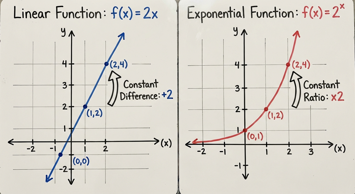
| Feature | Linear Function | Exponential Function |
|---|---|---|
| Change Type | Additive (Constant rate of change) | Multiplicative (Proportional rate of change) |
| Rule | $f(x)$ changes by adding a constant $m$ | $f(x)$ changes by multiplying by a factor $b$ |
| Form | $f(x) = mx + k$ | $f(x) = a(b)^x$ |
| Condition | Over equal input intervals $\Delta x$, differences in output $\Delta y$ are constant. | Over equal input intervals $\Delta x$, ratios of output $\frac{y2}{y1}$ are constant. |
AP Exam Tip: When analyzing a data table, check the inputs first! If inputs are not equally spaced, you must calculate the average rate of change (linear) or the growth factor per unit (exponential) to determine the model.
Exponential Functions
Exponential functions model unrestricted growth or decay. The general form is:
Where:
- $a$: The initial value (y-intercept) when $x=0$ (assuming no horizontal shift).
- $b$: The growth/decay factor (base). $b > 0$ and $b \neq 1$.
- $x$: The input variable.
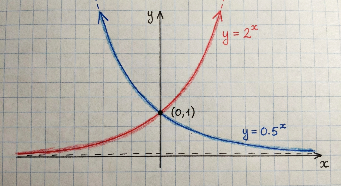
Growth vs. Decay
- Exponential Growth: $b > 1$.
- The function is always increasing (if $a > 0$).
- $\lim{x \to \infty} f(x) = \infty$ and $\lim{x \to -\infty} f(x) = 0$.
- Exponential Decay: $0 < b < 1$.
- The function is always decreasing (if $a > 0$).
- $\lim{x \to \infty} f(x) = 0$ and $\lim{x \to -\infty} f(x) = \infty$.
Concavity and Extremas
Exponential functions of the form $f(x) = ab^x$ express specific concavity behaviors:
- Extrema: They have no relative maxima or minima (no turning points) unless the domain is restricted to a closed interval.
- Inflection: They have no points of inflection. The concavity never changes.
- If $a > 0$: The graph is concave up for all real numbers.
- If $a < 0$: The graph is concave down for all real numbers (because it is reflected over the x-axis).
Transformations and Forms
- Rate form: $f(x) = a(1+r)^x$, where $r$ is the rate of growth/decay as a decimal.
- Horizontal Translation: $g(x) = b^{x+k}$. This is equivalent to a vertical dilation because $b^{x+k} = b^x \cdot b^k$, where $b^k$ becomes the new constant $a$.
- Horizontal Dilation: $g(x) = b^{cx}$. This changes the base of the function: $b^{cx} = (b^c)^x$. The new growth factor is $b^c$.
Composition and Inverse Functions
Composition of Functions
The composition $(f \circ g)(x) = f(g(x))$ maps inputs from $g$ through $g(x)$, and then uses that result as the input for $f$.
Implication: The range of the inner function $g(x)$ must fit within the domain of the outer function $f(x)$.
Inverse Functions
An inverse function $f^{-1}(x)$ reverses the mapping of $f(x)$.
- If $f(a) = b$, then $f^{-1}(b) = a$.
- Definition: Two functions are inverses if and only if $f(g(x)) = x$ and $g(f(x)) = x$ for all $x$ in their respective domains.
- Graphical Relationship: The graph of $f^{-1}(x)$ is the reflection of $f(x)$ across the line $y=x$.
- Domain/Range: The domain of $f$ becomes the range of $f^{-1}$, and the range of $f$ becomes the domain of $f^{-1}$.
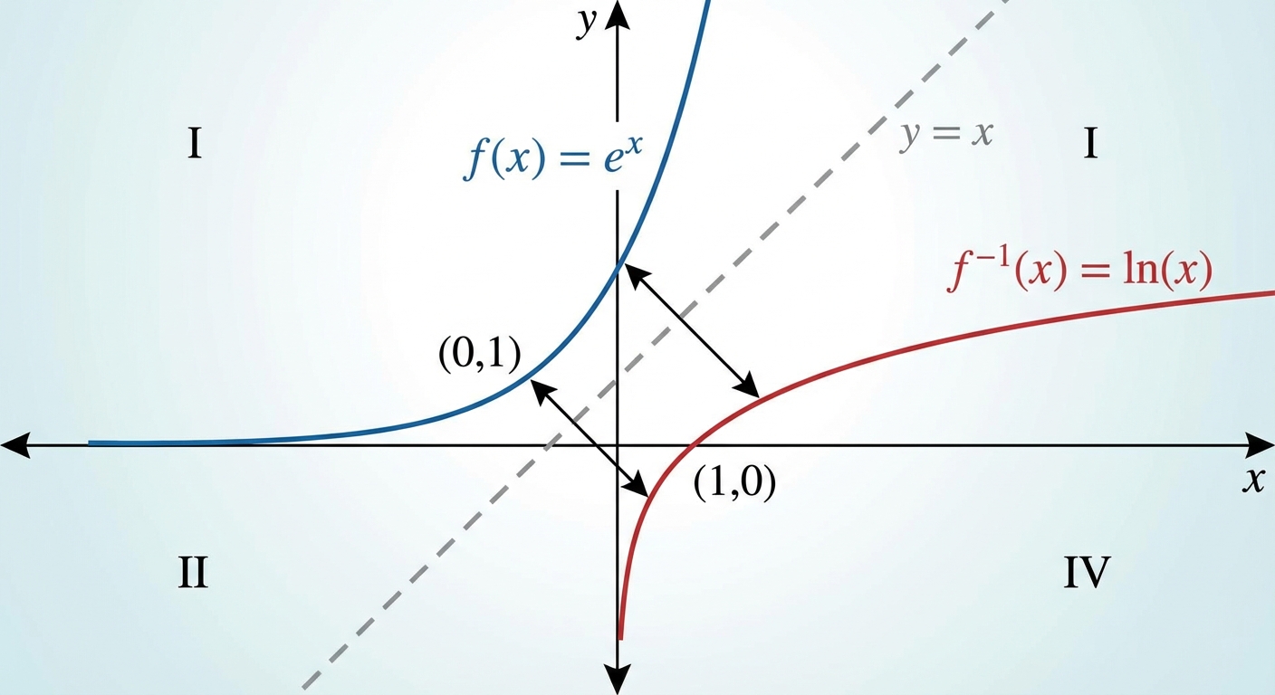
Logarithmic Functions
Logarithms are the inverses of exponential functions. They answer the question: "To what power must I raise base $b$ to get value $a$?"
Properties of Logarithms
Understanding these properties is essential for solving equations (Topic 2.13):
- Product Rule: $\logb(xy) = \logb(x) + \log_b(y)$
- Quotient Rule: $\logb\left(\frac{x}{y}\right) = \logb(x) - \log_b(y)$
- Power Rule: $\logb(x^n) = n \cdot \logb(x)$
- Change of Base: $\log_b(x) = \frac{\ln(x)}{\ln(b)} = \frac{\log(x)}{\log(b)}$
Graph Characteristics of $f(x) = \log_b(x)$
Since logs are inverses of exponentials, their features swap:
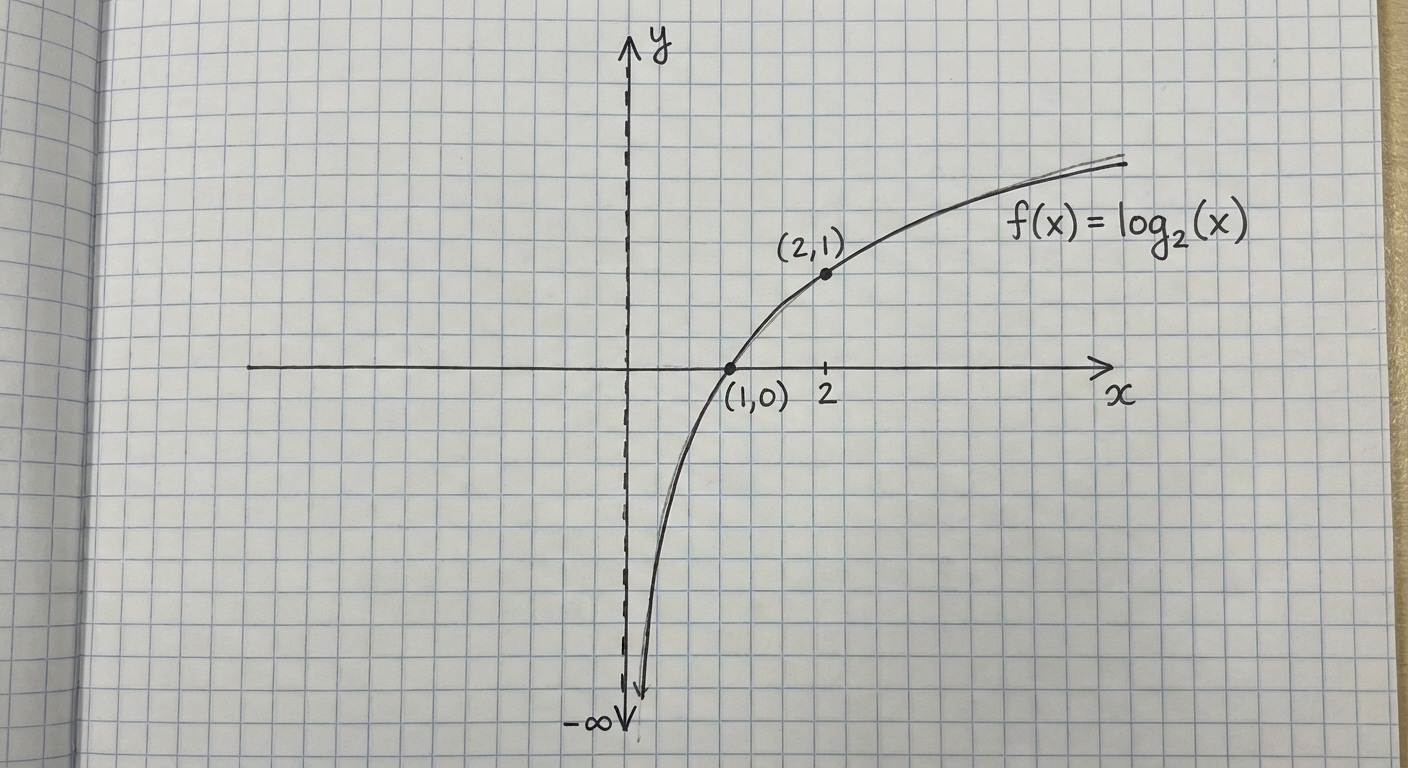
- Domain: $(0, \infty)$. Inputs must be positive.
- Range: $(-\infty, \infty)$. Outputs are all real numbers.
- Asymptote: Vertical asymptote at $x=0$ (exponentials have horizontal asymptotes).
- Concavity ($b > 1$):
- The function is increasing.
- The function is concave down (rate of increase slows down).
- Note: This is the inverse of exponential growth, which is increasing and concave up.
Logarithmic Growth vs. Exponential Growth
- Exponential: Input changes additively $\to$ Output changes multiplicatively.
- Logarithmic: Input changes multiplicatively $\to$ Output changes additively.
- Example: In $y = \log_2(x)$, if you double $x$ (multiply input), $y$ increases by exactly 1 (add to output).
Semi-Log Plots
(Topic 2.15)
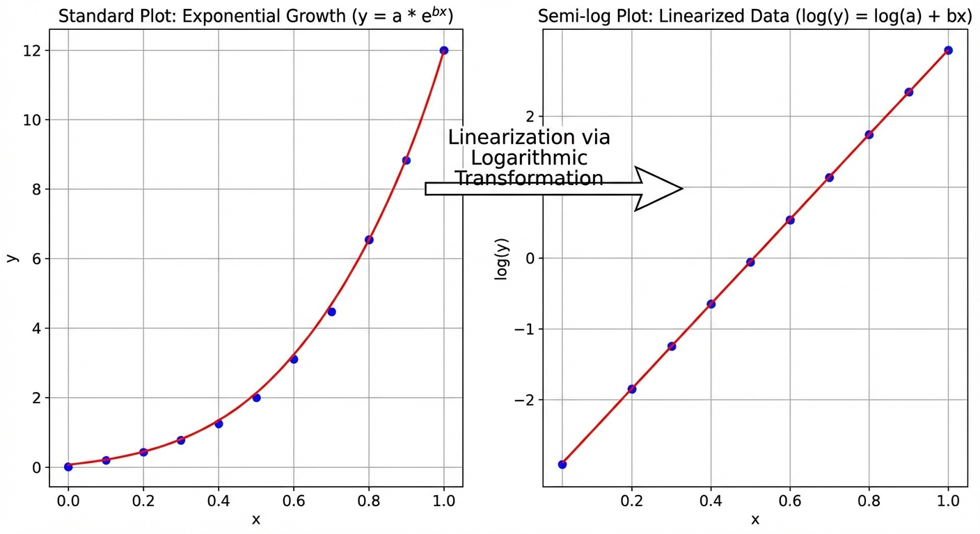
A semi-log plot is a graphing technique used to determine if data follows an exponential model and to linearize that data.
- Linearly Scaled Axis: Usually the input ($x$).
- Logarithmically Scaled Axis: Usually the output ($y$).
The Mathematical Logic
If a relationship is exponential ($y = ab^x$), applying a logarithm to both sides creates a linear equation:
This looks like the linear form $Y = mx + k$, where:
- The output variable is $Y = \log(y)$.
- The slope is $m = \log(b)$.
- The y-intercept is $k = \log(a)$.
Conclusion: If you plot $(x, \log y)$ and the points form a straight line, the original data is exponential.
Common Mistakes & Pitfalls
- Confusing Concavity: Students often forget that basic exponential growth ($b>1$) is concave up, while basic logarithmic growth ($b>1$) is concave down. A log function grows forever, but it grows slower and slower.
- Distributing Logarithms: A common error is writing $\log(a + b) = \log(a) + \log(b)$. This is false. The property applies to multiplication inside the log, not addition.
- Domain Errors: For $f(x) = \log_b(g(x))$, the domain requires $g(x) > 0$. Don't just set $g(x) \neq 0$.
- Inverse Notation: $f^{-1}(x)$ means inverse function, NOT $\frac{1}{f(x)}$ (reciprocal). The reciprocal is usually written as $[f(x)]^{-1}$.
- Solving Inequalities: When taking the log of both sides of an inequality with a base $0 < b < 1$, you must flip the inequality sign.