Analyzing Data through Linearization and Composition
Semi-Log Plots and Linearization
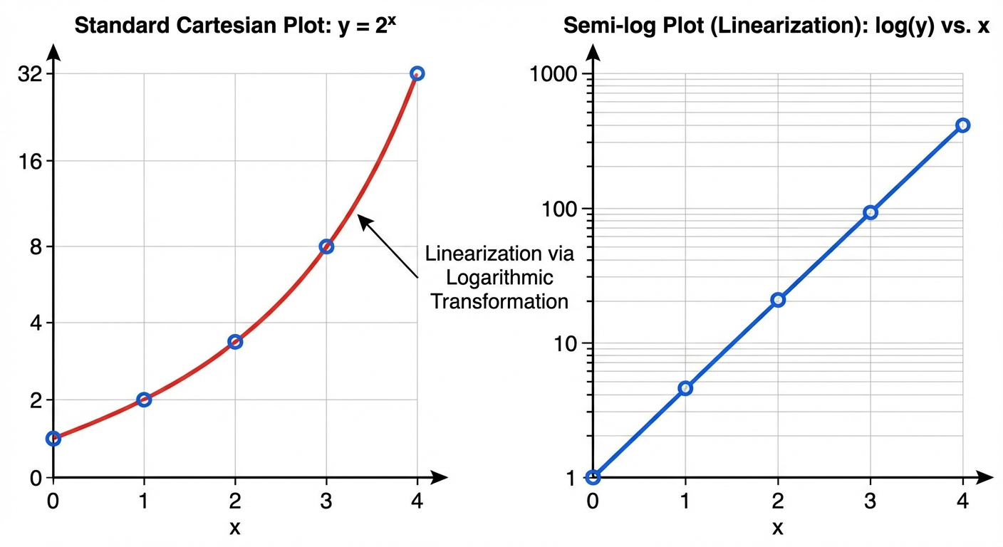
In science and mathematics, data often spans several orders of magnitude, or follows a non-linear growth pattern. A semi-log plot is a specialized graphing technique used to visualize exponential functions as straight lines. This process is often called linearization.
The Concept of Linearization
When you graph an exponential function like $y = ab^x$ on a standard Cartesian coordinate system (linear scales on both axes), the result is a curve. Determining specific parameters (like $a$ and $b$) just by looking at a curve is difficult.
However, if we transform the output values using logarithms, the exponential relationship transforms into a linear one. This allows us to use linear regression tools or simple slope calculations to model the data.
- Standard Plot: $x$ vs. $y$ produces a curve.
- Semi-Log Plot: $x$ vs. $\log(y)$ (or $\ln(y)$) produces a straight line.
Deriving the Linear Form
To understand why this works, we apply properties of logarithms to the standard exponential equation.
Starting with the exponential model:
Take the logarithm (natural or base 10) of both sides:
Apply the product rule of logarithms ($\ln(mn) = \ln m + \ln n$):
Apply the power rule of logarithms ($\ln(x^p) = p \ln x$):
Rearrange to look like the slope-intercept form ($Y = mx + k$):
In this linearized equation:
- The input represents $x$.
- The output represents $\ln(y)$ (the log of the original data).
- The slope ($m$) represents $\ln(b)$ (the log of the growth factor).
- The y-intercept ($k$) represents $\ln(a)$ (the log of the initial value).
Analyzing Data from Semi-Log Plots
If you are given a data set or a graph where the $y$-axis is on a logarithmic scale and the data forms a line, you can conclude the underlying relationship is exponential.
Steps to Find the Exponential Equation:
- Calculate the Linear Equation: Find the slope ($m$) and y-intercept ($k$) of the line using the points $(x1, \log y1)$ and $(x2, \log y2)$.
- Solve for the Base ($b$): Since $m = \ln b$ (or $\log b$), use the inverse log property:
- Solve for the Coefficient ($a$): Since $k = \ln a$:
Modeling with Exponential and Logarithmic Functions
Mathematical modeling involves choosing a function that behaves similarly to a real-world phenomenon. In AP Precalculus, you must distinguish between scenarios that require exponential models versus those that require logarithmic models.
Determining the Model Type
| Function Type | General Form | Data Characteristic |
|---|---|---|
| Exponential | $y = a(b)^x$ | As $x$ increases by a constant amount (arithmetic), $y$ changes by a constant ratio (geometric). Used for populations, radioactive decay, interest. |
| Logarithmic | $y = a + b \ln(x)$ | As $x$ increases by a constant ratio (geometric), $y$ changes by a constant amount (arithmetic). Used for pH levels, decibels, magnitude scales. |
Concavity and Growth Rates
When looking at a scatterplot or data table, the concavity and rate of change help identify the function.
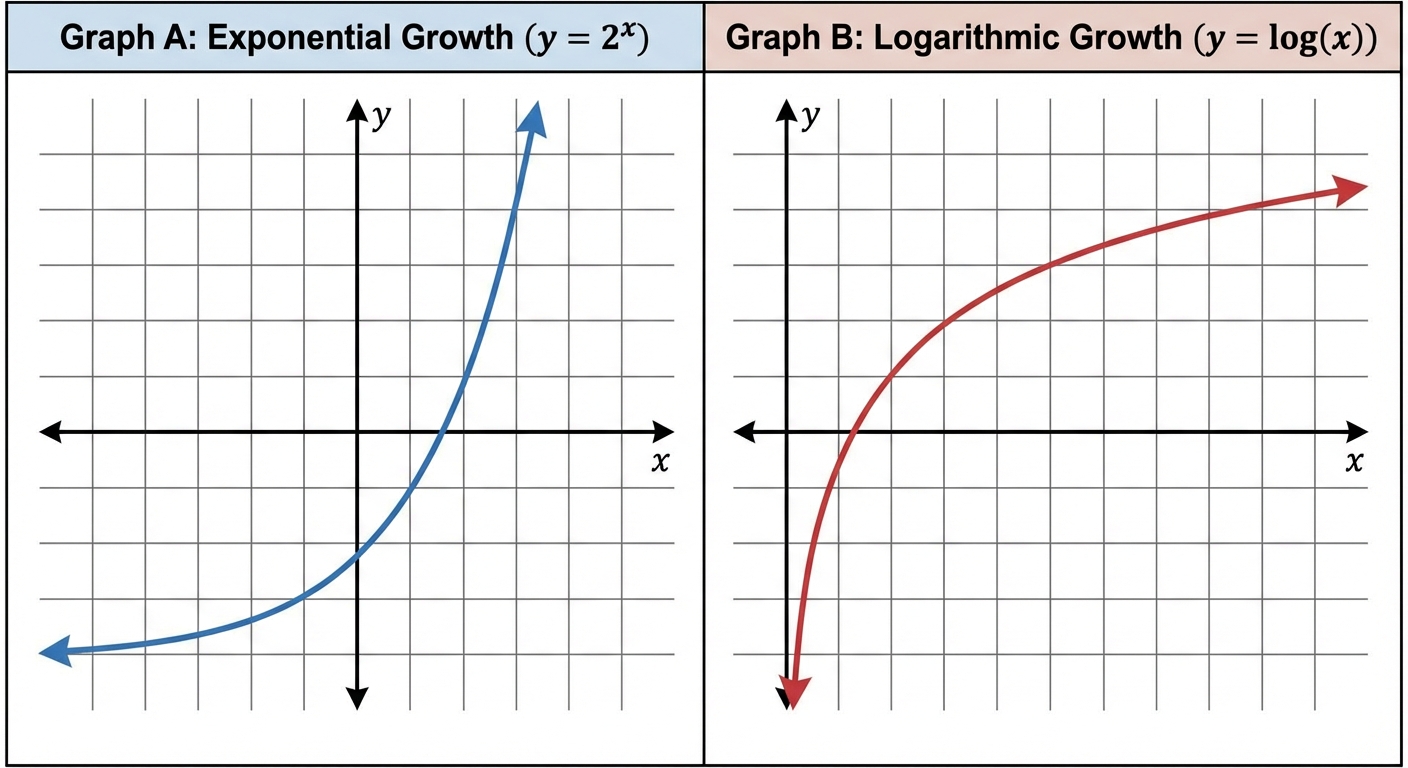
- Exponential Growth ($b > 1$): Increasing and concave up. The rate of change increases rapidly as $x$ increases.
- Logarithmic Growth ($b > 0$): Increasing and concave down. The rate of change decreases (slows down) as $x$ increases, but the function theoretically grows without bound.
Worked Example: Modeling from Data
Problem: A researcher collects the following data:
| $t$ (hours) | $0$ | $2$ | $4$ |
|---|---|---|---|
| $V(t)$ | $50$ | $140$ | $392$ |
Solution:
- Check for Equal Intervals: The input $t$ increases by 2 every step (arithmetic).
- Check Ratios: Calculate the ratio of consecutive outputs:
- Conclusion: Since the ratios are constant, this is an exponential model.
- Form: $V(t) = a \cdot b^t$.
- At $t=0$, $V(0) = 50$, so $a = 50$.
- Since the interval is 2 hours, the growth over 2 hours is $2.8$. So $b^2 = 2.8 \implies b = \sqrt{2.8} \approx 1.673$.
- Model: $V(t) = 50(1.673)^t$.
Composition of Exponential and Logarithmic Functions
Function composition involves substituting one function into another, denoted as $f(g(x))$. When combining exponential and logarithmic functions, compositions often utilize inverse properties to simplify expressions or model complex behaviors.
Inverse Properties
Because $f(x) = b^x$ and $g(x) = \log_b x$ are inverse functions, their compositions cancel out, leaving the argument unchanged (provided the domain is valid).
- $\log_b(b^x) = x$
- $b^{\log_b x} = x$ (for $x > 0$)
Modeling with Composition
Composition is frequently used to transform variables or combine rates.
Example: Atmospheric Pressure
Let input $h$ be altitude in kilometers. The pressure $P$ in millibars decreases exponentially: $P(h) = 1000(0.88)^h$.
Suppose altitude $h$ depends on time $t$ effectively linearly as a weather balloon rises: $h(t) = 0.5t$.
The pressure with respect to time is a composition $P(h(t))$:
Domain and Range of Compositions
When finding the domain of $f(g(x))$:
- $x$ must be in the domain of the inner function $g(x)$.
- The output $g(x)$ must be in the domain of the outer function $f(x)$.
Example: Let $f(x) = \log(x)$ and $g(x) = 4 - x^2$.
Find the domain of $f(g(x)) = \log(4 - x^2)$.
- Constraint: The argument of the log must be positive.
- $4 - x^2 > 0$
- $-x^2 > -4 \implies x^2 < 4$
- Domain: $(-2, 2)$.
Common Mistakes & Pitfalls
Confusing Plot Axes for Linearization:
- Mistake: Thinking that plotting $\log x$ vs. $\log y$ linearizes an exponential function.
- Correction: $\log x$ vs. $\log y$ linearizes a Power Function ($y=ax^p$). For Exponential Functions ($y=ab^x$), you must plot $x$ vs. $\log y$ (semi-log).
Misinterpreting the Slope on a Semi-Log Plot:
- Mistake: Assuming the measured slope of the linearized data is the base $b$.
- Correction: The slope of the line is $\ln(b)$ (or $\log(b)$ depending on the base used). You must exponentiate the slope to find the actual growth factor: $b = e^{slope}$.
Domain Violations in Composition:
- Mistake: Canceling out functions without checking constraints, e.g., claiming $e^{\ln(-5)} = -5$.
- Correction: The domain of $\ln(x)$ is $(0, \infty)$. You cannot take the log of a negative number, so the expression is undefined, not $-5$.