Mastering Problem-Solving and Data Analysis on the SAT
Quantitative Reasoning and Data Interpretation
The "Problem-Solving and Data Analysis" section of the SAT Math test assesses your ability to use math in real-world situations. It is less about abstract algebra and more about being data-literate: understanding ratios, interpreting graphs, and making logical inferences from statistics.
Ratios, Rates, and Proportions
These problems often involve unit conversions, density, or comparing quantities. The core skill here is Dimensional Analysis (keeping track of your units).
Unit Conversion and Rates
When converting units, arrange your conversion factors so that unwanted units cancel out.
Key Concepts:
- Rate: A ratio comparing two different units (e.g., miles per hour, dollars per pound).
- Density: A specific type of rate defined as mass per unit volume ($Density = \frac{m}{v}$) or population per unit area.
Proportional Relationships
Two quantities, $x$ and $y$, are directly proportional if $y = kx$, where $k$ is the constant of proportionality.
Example Scenario:
If a printer prints 40 pages in 5 minutes, how many pages does it print in 12 minutes?
- Calculate the unit rate: $\frac{40 \text{ pages}}{5 \text{ min}} = 8 \text{ pages/min}$.
- Apply to new time: $8 \text{ pages/min} \times 12 \text{ min} = 96 \text{ pages}$.
Percentages
Percentages are heavily tested, specifically how to model increases and decreases efficiently.
The Multiplier Method
Instead of calculating the percentage amount and adding it back, use a single multiplier.
- Percent Increase: To increase a number $x$ by $p$%, multiply by $(1 + \frac{p}{100})$.
- Example: Increasing by 20% $\rightarrow$ multiply by $1.20$.
- Percent Decrease: To decrease a number $x$ by $p$%, multiply by $(1 - \frac{p}{100})$.
- Example: Decreasing by 15% $\rightarrow$ multiply by $0.85$.
Percent Change Formula
When asked for the percent change between an original value and a new value:
Common Mistake Alert: Always ensure the denominator is the original (or starting) value, not the new value.
Analyzing One-Variable Data
This section deals with summarizing a single list of numbers (like test scores or heights) using measures of center and spread.
Measures of Center
- Mean (Average): The sum of data points divided by the count.
- Median: The middle value when data is ordered from least to greatest. If there is an even number of points, average the two middle numbers.
- Mode: The most frequently occurring value.
Comparisons and Outliers
- Outliers: Extreme values used to skew data.
- Resistance: The Median is resistant to outliers (it won't move much). The Mean is NOT resistant to outliers (it will be pulled toward the extreme value).
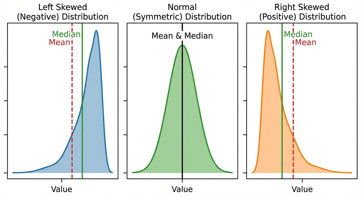
- Skewed Right (Positive): The tail extends to the right (high values). Mean $>$ Median.
- Skewed Left (Negative): The tail extends to the left (low values). Mean $<$ Median.
- Symmetric: Mean $\approx$ Median.
Measures of Spread
- Range: .
- Standard Deviation (SD): Measures the average distance of data points from the mean. You do not need to calculate SD, but you must conceptually compare it.
- Data points clustered extensively near the mean = Low SD.
- Data points spread out far from the mean = High SD.
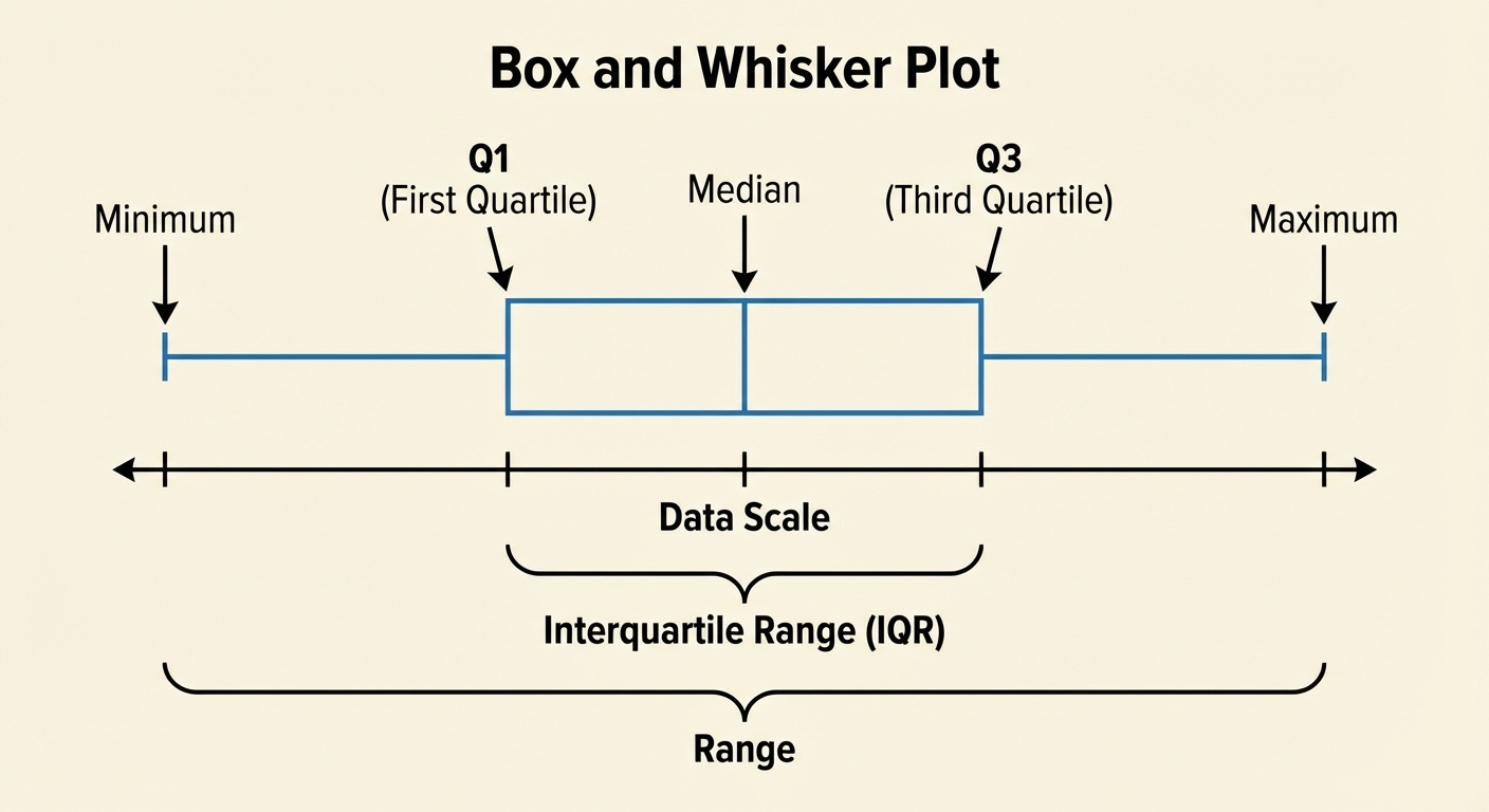
Box Plots (Box-and-Whisker)
A box plot visually displays the "Five Number Summary": Min, Q1 (25th percentile), Median (50th percentile), Q3 (75th percentile), and Max.
Two-Variable Data and Scatterplots
Here, we analyze the relationship between two variables, typically $x$ and $y$.
Line of Best Fit
The SAT creates a model (usually linear) to describe the trend in data: $y = mx + b$.
- Slope ($m$): The rate of change. It tells you how much $y$ changes for every one unit increase in $x$.
- Y-intercept ($b$): The value of $y$ when $x$ is 0. often representing the "starting amount" or "initial value."
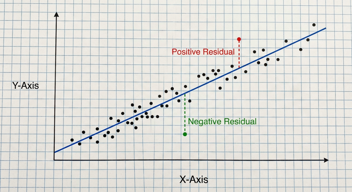
Residuals
A residual is the difference between the actual data point and the predicted value (the line).
- Positive residual: The data point is above the line.
- Negative residual: The data point is below the line.
Linear vs. Exponential Models
- Linear Growth: Increases by a constant amount (e.g., adding 5 every year).
- Exponential Growth: Increases by a constant percentage or factor (e.g., doubling every year).
Probability and Conditional Probability
Probability on the SAT is almost always based on data tables (two-way tables).
Basic Probability
Conditional Probability
This asks for the probability of an event given a specific condition. This restricts your denominator.
Example Logic:
"Given that a selected person is over 65, what is the probability they voted?"
- Denominator: Total number of people over 65 (NOT the total population).
- Numerator: People who are over 65 AND voted.
Inferential Statistics and Study Design
This topic tests if you understand what makes a valid scientific conclusion.
Sample vs. Population
- Population: The entire group you want to know about.
- Sample: The subset of the group you actually measure.
The Golden Rules of Inference
- Random Selection: If participants are chosen randomly from a population, the results can be generalized to that population.
- Random Assignment: If participants are randomly assigned to treatment/control groups, you can infer cause and effect.
| Condition | What you can claim |
|---|---|
| Observational Study | Correlation (Association) only. No causation. |
| Controlled Experiment | Causation (if variables are controlled). |
Margin of Error
The margin of error describes the uncertainty of a sample statistic.
- Sample Size Rule: To decrease the margin of error, you must increase the sample size.
- The variability of the data also affects it: more variable data = larger margin of error.
Common Mistakes & Pitfalls
- Percent Change Denominator: When a price goes from \$50 to \$80, the increase is $\frac{30}{50}$, not $\frac{30}{80}$. Always divide by the starting number.
- Misinterpreting Slope: Don't just say "slope is rise over run." Interpret it in context: "For every additional hour studied, the score increases by 10 points."
- Confusion with "Mean" vs "Median": remember that if a graph has a long tail to the right (rich people in a neighborhood), the Mean is pulled higher than the Median.
- Correlation vs. Causation: Just because ice cream sales and shark attacks both go up in summer doesn't mean ice cream causes shark attacks. Without a controlled experiment, you cannot claim causation.
- Unit Blindness: If a speed is in feet per second but the time is in minutes, you MUST convert before multiplying.