Foundations of Firm Behavior: Production and Cost Analysis
The Production Function
To understand how firms make decisions, we must first analyze the engineering relationship between inputs (resources) and outputs (goods). This relationship is called the Production Function.
Time Horizons: Short Run vs. Long Run
In economics, the distinction between the short run and long run is not defined by a specific calendar time (e.g., "one year"), but by the flexibility of inputs.
- Short Run: A period in which at least one input is fixed (cannot be changed). usually, Capital ($K$) (like factory size or machinery) is fixed, while Labor ($L$) is variable.
- Long Run: A period in which all inputs are variable. The firm can alter plant size, buy new machines, or exit the industry entirely.
Key Production Metrics
To analyze production, we track three specific measures:
- Total Product ($TP$): The total quantity of output produced with a given amount of inputs.
- Marginal Product ($MP$): The additional output generated by adding one more unit of a variable input (usually labor).
- Average Product ($AP$): The output produced per unit of variable input.
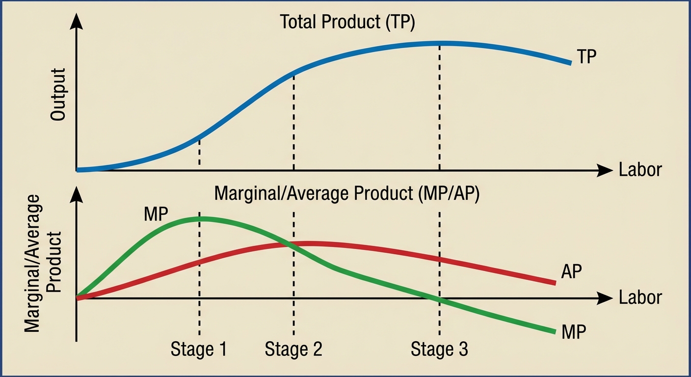
The Law of Diminishing Marginal Returns
This is the governing principle of Short-Run production. It states that as you add variable resources (Labor) to distinct fixed resources (Capital), the additional output produced from each new worker will eventually fall.
- Stage I (Increasing Returns): Specialization allows workers to be more efficient. $MP$ is rising.
- Stage II (Diminishing Returns): The fixed capital becomes crowded. Each new worker adds to $TP$, but less than the previous worker. $MP$ is positive but falling.
- Stage III (Negative Returns): The factory is so overcrowded that workers get in each other's way. $TP$ actually falls. $MP$ is negative.
The Relationship Between MP and AP
Think of this like your Grade Point Average (GPA). Marginal Product drives Average Product.
- If $MP > AP$, then $AP$ is rising (the new worker pulls the average up).
- If $MP < AP$, then $AP$ is falling (the new worker drags the average down).
- Geometric Rule: The $MP$ curve intersects the $AP$ curve at the maximum of the $AP$ curve.
Short-Run Production Costs
Once a firm understands its production numbers, it applies prices to those inputs to determine costs. Costs in microeconomics include both Explicit Costs (out-of-pocket money payments) and Implicit Costs (opportunity costs of owned resources).
Categorizing Total Costs
In the short run, costs are split based on whether the input is fixed or variable.
- Fixed Costs ($FC$): Costs that do not change with output quantity. You pay these even if you produce 0 units (e.g., Rent, Insurance).
- Variable Costs ($VC$): Costs that increase as output increases (e.g., Wages, Raw Materials).
- Total Cost ($TC$): The sum of fixed and variable costs.
Per-Unit Costs (Average and Marginal)
These are the most critical curves for AP Microeconomics graphing.
- Marginal Cost ($MC$): The additional cost of producing one more unit of output.
- Average Fixed Cost ($AFC$): Fixed cost per unit.
- Average Variable Cost ($AVC$): Variable cost per unit.
- Average Total Cost ($ATC$): Total cost per unit.
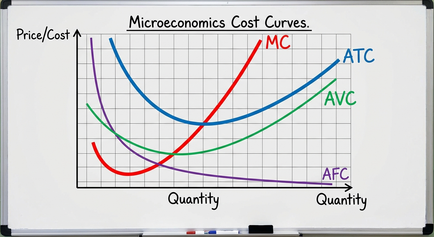
Graphical Relationships & Rules
- The Check-Mark Shape: The $MC$ curve falls initially (due to specialization) and then rises steeply due to Diminishing Marginal Returns.
- Intersection Points: The $MC$ curve intersects both the $ATC$ and the $AVC$ minimum points. (Similar to the GPA analogy: if the cost of the next unit is cheaper than the average, the average drops).
- Vertical Distance: The vertical distance between $ATC$ and $AVC$ represents the $AFC$. As Quantity ($Q$) increases, $AFC$ gets smaller, so $ATC$ and $AVC$ get closer together but never touch.
| Quantity ($Q$) | Fixed Cost ($TFC$) | Variable Cost ($TVC$) | Total Cost ($TC$) | Marginal Cost ($MC$) | $ATC$ | $AVC$ |
|---|---|---|---|---|---|---|
| 0 | $100 | $0 | $100 | - | - | - |
| 1 | $100 | $20 | $120 | $20 | $120 | $20 |
| 2 | $100 | $35 | $135 | $15 | $67.5 | $17.5 |
| 3 | $100 | $60 | $160 | $25 | $53.3 | $20 |
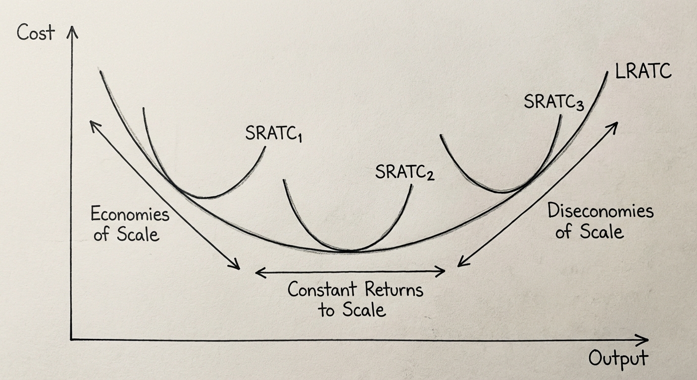
Long-Run Costs and Returns to Scale
In the Long Run, there are no fixed costs. The firm can change all inputs. The curve that connects the lowest possible cost of producing any given quantity in the long run is the Long-Run Average Total Cost (LRATC) curve.
Scales of Production
The shape of the LRATC curve is U-shaped, but for different reasons than the short-run ATC.
- Economies of Scale: As the firm gets larger, long-run average costs fall. This happens due to bulk buying, management specialization, and better technology usage.
- Graphically: The downward-sloping section of LRATC.
- Constant Returns to Scale: Average costs remain constant as output increases.
- Graphically: The flat bottom section of LRATC.
- Diseconomies of Scale: As the firm gets too massive, long-run average costs rise. This occurs due to bureaucracy, communication failures, and management inefficiency.
- Graphically: The upward-sloping section of LRATC.
Math of Returns to Scale
If a firm doubles ALL inputs (e.g., $2x$ Labor and $2x$ Capital):
- Increasing Returns to Scale: Output more than doubles.
- Constant Returns to Scale: Output exactly doubles.
- Decreasing Returns to Scale: Output less than doubles.
(Note: "Returns to Scale" refers to Production; "Economies of Scale" refers to Cost. They are inverse sides of the same coin.)
Summary of Common Mistakes
1. Diminishing Returns vs. Diseconomies of Scale
- Mistake: Using these terms interchangeably.
- Correction: Diminishing Marginal Returns is a Short-Run concept caused by fixed resources. Diseconomies of Scale is a Long-Run concept caused by coordination issues.
2. Shifts in Cost Curves
- Mistake: Moving the whole curve when only quantity changes.
- Rule:
- A change in Fixed Costs (e.g., Rent goes up) shifts $AFC$ and $ATC$ upward. $MC$ and $AVC$ do not change.
- A change in Variable Costs (e.g., Wages go up) shifts $MC$, $AVC$, and $ATC$ upward. $AFC$ does not change.
3. The Relationship between Total and Marginal
- Mistake: Thinking Peak Total Product is where Marginal Product is highest.
- Correction: When Total Product is at its maximum, Marginal Product is zero. If you add one more worker, MP becomes negative and Total Product falls.
Memory Mnemonic: The "Nike" Swoosh
When drawing cost curves, remember the shape of the Marginal Cost ($MC$) curve looks like a Nike swoosh (check mark). It always cuts the "U" family ($ATC$ and $AVC$) at their lowest points.