Advanced Dynamics: Resistive and Elastic Forces
Topic Overview
In AP Physics C: Mechanics, simply knowing Newton's Second Law ($\Sigma \vec{F} = m\vec{a}$) is not enough. You must understand how to apply it to dynamic forces that change based on conditions like contact surface properties, velocity, and position. This section covers the three primary variable forces you will encounter: Friction, Drag, and Spring Forces.
Friction Forces
Friction is a resistive force that arises from the microscopic interactions between two surfaces in contact. It always acts parallel to the surface interface and opposes the direction of relative motion (or impending motion).
Static vs. Kinetic Friction
There are two distinct regimes of friction. It is crucial to determine whether an object is moving relative to the surface or remaining stationary.
- Static Friction ($f_s$): Acts when surfaces are not sliding relative to each other. It is a "smart" force that matches the applied force exactly to keep the object in equilibrium, up to a maximum limit.
- Kinetic Friction ($f_k$): Acts when surfaces are sliding relative to each other. It is generally constant for a given pair of surfaces and is usually weaker than the maximum static friction.
The relationship between friction and the Normal Force ($F_N$) is governed by the coefficient of friction ($\mu$), a unitless scalar determined by surface roughness.
Formulas
| Force Type | Formula | Characteristic |
|---|---|---|
| Static Friction | An inequality. The force ranges from $0$ to $f_{s,max}$. | |
| Max Static | f_{s,max} = | |
| us FN | The "breaking point" just before slipping occurs. | |
| Kinetic Friction | A constant value once motion begins (usually $\muk < \mus$). |
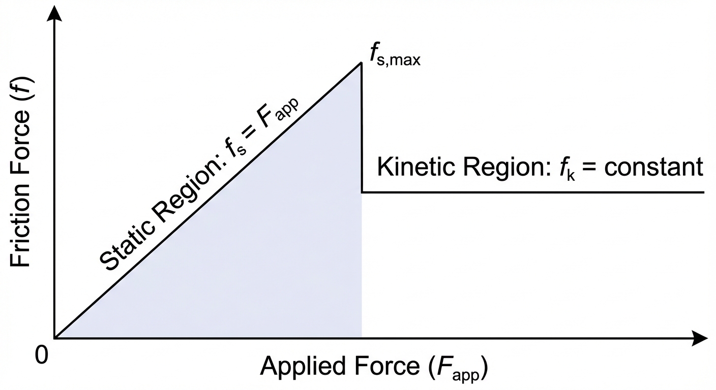
Graphical Representation
When you apply an increasing external force to a stationary block, the friction force increases linearly (slope = 1) to match the push. Once the maximum static limit is reached, the object "breaks free," and the force drops instantly to the lower, constant kinetic friction level.
Worked Example: The Inclined Plane
Scenario: A block of mass $m$ sits on a ramp inclined at angle $\theta$. The coefficient of static friction is $\mus$. What is the critical angle $\thetac$ where the block just begins to slip?
Solution:
- Define Coordinates: Tilt the axes so $x$ is parallel to the ramp (downward) and $y$ is perpendicular.
- Forces:
- Gravity: $mg \sin\theta$ (down the ramp), $mg \cos\theta$ (into the ramp).
- Normal Force: $F_N$ (out of the ramp).
- Friction: $f_s$ (up the ramp, opposing potential slip).
- Newton's Second Law ($ {acceleration} = 0$):
- y-axis: $FN - mg \cos\theta = 0 \implies FN = mg \cos\theta$
- x-axis: $mg \sin\theta - fs = 0 \implies fs = mg \sin\theta$
- Apply Threshold Condition: Just before slipping, $fs = f{s,max} = \mus FN$.
- Substitute and Solve:
Drag Forces and Terminal Velocity
Unlike friction (which depends on the normal force), drag ($F_D$) is a resistive force exerted by a fluid (liquid or gas) that depends on the velocity of the object. Drag always acts opposite to the velocity vector.
Regimes of Drag
- Linear Drag (Low Speed / Laminar): Common for small objects moving slowly (e.g., dust in air, ball bearing in oil).
- Quadratic Drag (High Speed / Turbulent): Common for large objects moving quickly (e.g., skydivers, baseballs).
(Note: The negative sign indicates direction opposite to velocity)
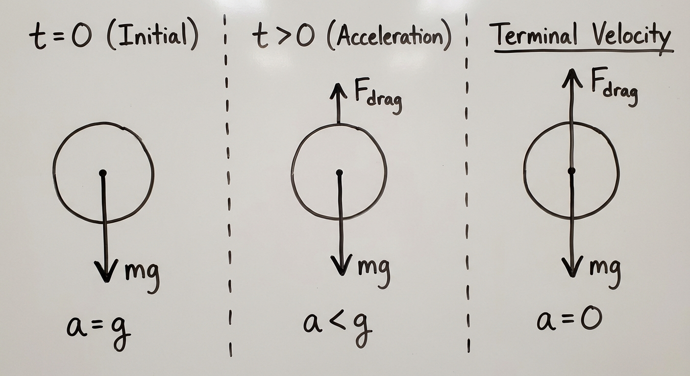
Terminal Velocity ($v_T$)
As an object falls, gravity is constant, but drag increases as speed increases. Eventually, the drag force equals the gravitational force. At this point, the net force is zero, acceleration is zero, and the velocity becomes constant. This is Terminal Velocity.
For a falling object with linear drag:
Calculus Application: Deriving Velocity as a Function of Time
In AP Physics C, you must be able to use differential equations to find velocity over time. Let's look at an object dropping from rest using Linear Drag ($F_D = -bv$).
Set up Newton's Second Law:
Separate Variables: Get all $v$ terms on one side and $t$ terms on the other.
Integrate both sides: (Limits: $v=0$ to $v(t)$, time $0$ to $t$)
Solve (u-substitution let $u = mg-bv$):
Exponentiate:
Result: The velocity approaches $mg/b$ asymptotically as $t \to \infty$.
Spring Forces (Hooke's Law)
Springs exert a Restoring Force. This means the force is always directed toward the spring's equilibrium position (where it is neither stretched nor compressed).
Hooke's Law
For an ideal spring, the force is proportional to the displacement from equilibrium.
- $k$: Spring constant (Units: N/m). Represents stiffness; a higher $k$ means a stiffer spring.
- $x$: Displacement from the equilibrium position ($x=0$).
- Minus sign: Critical! It indicates the force opposes the displacement.
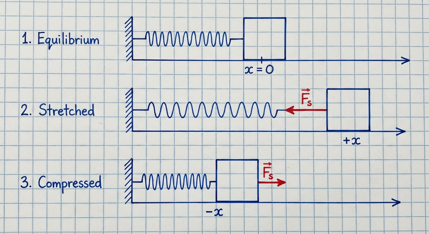
Visualizing Displacement
- If you pull the spring to the right ($+x$), the spring pulls back to the left ($-F$).
- If you compress the spring to the left ($-x$), the spring pushes back to the right ($+F$).
Non-Ideal Springs
In reality, springs stop obeying Hooke's law if stretched too far (plastic deformation). However, for AP Physics C Mechanics, assume springs are ideal and massless unless stated otherwise.
Common Mistakes & Pitfalls
1. The "Normal Force Trap"
Mistake: Assuming $FN = mg$ automatically. Correction: $FN$ is a reaction force. It changes based on the angle of the surface, applied vertical forces, or vertical acceleration (e.g., an elevator). Always solve for $FN$ using $\Sigma Fy = ma_y$.
2. Static Friction Misconception
Mistake: Assuming static friction always equals $\mus FN$.
Correction: $\mus FN$ is the maximum possible static friction. If you push a fridge with 10N and it doesn't move, static friction is exactly 10N, even if the maximum could be 500N. Do not use the maximum formula unless the problem states slipping is "impending" or the object is on the verge of moving.
3. Drag Acceleration
Mistake: Thinking acceleration is constant for falling objects with drag.
Correction: Acceleration is not constant. As velocity increases, drag increases, which decreases the net force. Therefore, acceleration decreases over time until it hits zero at terminal velocity.
4. Hooke's Law Sign Conventions
Mistake: Dropping the negative sign in $\vec{F} = -k\vec{x}$ when setting up differential equations.
Correction: The negative sign is crucial for defining simple harmonic motion (Unit 5), but even in Unit 2, ensure your force vector points opposite to the displacement vector.