AP Calculus AB Unit 1: Limits and Continuity (Comprehensive Study Guide)
What a Limit Means (and Why Calculus Starts Here)
The core idea
At its core, calculus is the study of change. Before determining instantaneous change (derivatives), we must understand how functions behave as inputs get close to specific values.
A limit describes what value a function’s output is approaching as the input approaches a particular number. The key word is approaching: limits are about trends, not necessarily what happens exactly at the point.
When you write
you are saying: as %%LATEX1%% gets closer and closer to %%LATEX2%% (without needing to equal %%LATEX3%%), the values of %%LATEX4%% get closer and closer to %%LATEX5%%. Crucially, limits do not care what happens at %%LATEX6%%, only what happens around it.
This matters because derivatives (rates of change) and integrals (accumulated change) both depend on limits.
Limit value vs. function value
A common early confusion is mixing up %%LATEX7%% with %%LATEX8%%. A helpful way to remember it is: the limit is about the journey (approach); the function value is the destination.
- %%LATEX9%% is the actual output when you plug in %%LATEX10%%.
- %%LATEX11%% is what the outputs approach near %%LATEX12%%.
They can be the same, but they don’t have to be. A function might have a “hole” at %%LATEX13%% where %%LATEX14%% is undefined, but the nearby values still approach a specific number. In that case the limit can exist even though the function value doesn’t.
Two-sided limits and one-sided limits
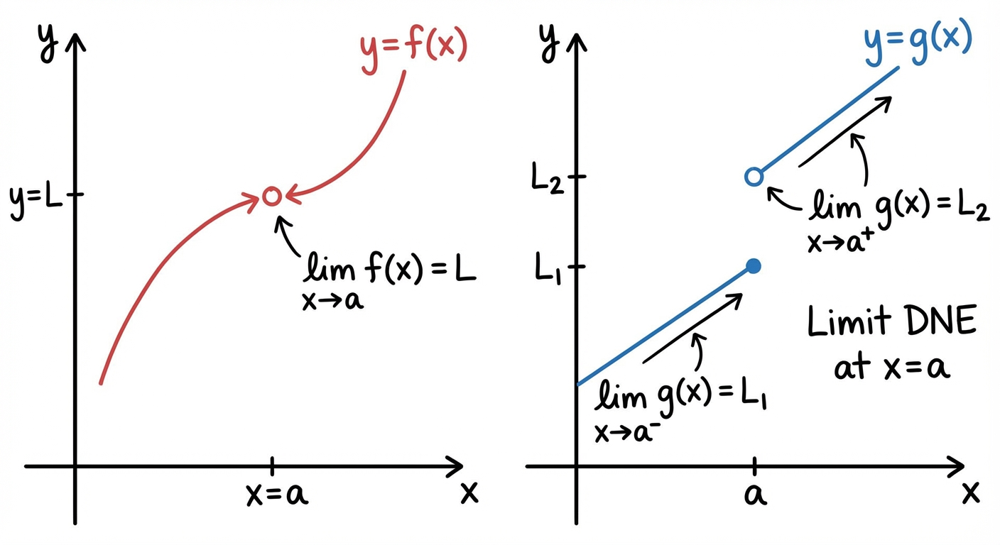
A two-sided limit looks at what happens as you approach from both directions.
means the left-hand and right-hand behavior both approach the same number.
The left-hand limit approaches %%LATEX16%% from values less than %%LATEX17%%:
The right-hand limit approaches %%LATEX19%% from values greater than %%LATEX20%%:
A two-sided limit exists exactly when both one-sided limits exist and are equal.
The General Limit Existence Theorem
The two-sided limit exists (and equals ) if and only if both one-sided limits exist and match:
if and only if
If the left and right approaches do not match, the limit does not exist (DNE).
When limits fail to exist
It’s not “bad” if a limit doesn’t exist; it just means the approach behavior isn’t settling to a single number. Common reasons:
- Jump behavior: left-hand and right-hand limits are different.
- Infinite behavior: values grow without bound near the point (vertical asymptote behavior).
- Oscillation: values keep flipping around without approaching one number (like certain sine-based constructions near ).
Notation reference (same idea, different looks)
| Concept | Common notation | What it means |
|---|---|---|
| Two-sided limit | Approach from both sides | |
| Left-hand limit | Approach from the left | |
| Right-hand limit | Approach from the right | |
| Limit equals | The approached output value |
Worked example: limit vs. function value
Suppose a function is defined as follows:
- For inputs close to %%LATEX33%% (but not equal to %%LATEX34%%), the graph lies on the line .
- At %%LATEX36%%, the function is instead defined to be %%LATEX37%%.
Then the approaching behavior near %%LATEX38%% is still governed by %%LATEX39%%, so
But the actual value is
So the limit and the function value differ.
Worked example: one-sided limits determine existence
Imagine approaching :
- From the left, values approach .
- From the right, values approach .
Then
and
Because these are not equal, the two-sided limit does not exist:
Exam Focus
- Typical question patterns:
- Given a graph, report %%LATEX48%%, %%LATEX49%%, %%LATEX50%%, and %%LATEX51%%.
- Decide whether a limit exists and justify using one-sided limits.
- Interpret limit notation in words (“approaches,” not “equals”).
- Common mistakes:
- Assuming automatically.
- Forgetting a two-sided limit requires both one-sided limits to match.
- Mixing up the meaning of the minus sign in a one-sided limit. For example, means “approach 2 from the left,” not “approach negative 2.”
- Saying “the limit is infinity” as if %%LATEX54%% were a normal number. AP typically expects language like “diverges to %%LATEX55%%” or “does not exist as a finite number.”
Estimating Limits from Graphs and Tables
Reading limits from graphs (the right mindset)
When you estimate a limit from a graph, you are doing a visual version of “getting close.” A good strategy is to literally trace the curve with your finger toward %%LATEX56%% from the left and from the right and watch where the %%LATEX57%%-values head.
Two important reminders:
- The point at might be an open circle, a filled dot somewhere else, or not shown at all. The limit only cares about the approach, not the plotted value at the point.
- If the left and right sides approach different heights, the two-sided limit does not exist.
Holes, jumps, and asymptotes on graphs
- Removable discontinuity (hole): The graph approaches a single height from both sides, but there is an open circle (and maybe a filled dot elsewhere). The limit exists. (On a graph, the limit is the y-value of the hole.)
- Jump discontinuity: The graph approaches one height from the left and a different height from the right. The two-sided limit does not exist.
- Vertical asymptote behavior: The graph shoots upward or downward near . The limit is not a finite number; the function is unbounded near that point.
If the graph rises without bound as , you may write
If it decreases without bound, you may write
Sometimes a vertical asymptote has different one-sided behavior, so the two-sided limit may be described one-sidedly, or you may say it DNE as a finite value (and specify the one-sided infinite limits).
Estimating limits from tables
A table is a numerical snapshot: you look at values of %%LATEX63%% for %%LATEX64%% close to . A good table for limits includes values approaching from both sides:
- values slightly less than
- values slightly greater than
You are not looking for where %%LATEX68%% equals %%LATEX69%%; you are looking for the trend as gets closer.
A subtle issue: rounding can hide behavior. If values are very large (positive or negative) or change erratically, that’s a hint the limit may not be a finite number or may not exist.
Example: estimating a limit from a table (approaching a finite value)
Suppose you are given values near :
- When %%LATEX72%%, %%LATEX73%%
- When %%LATEX74%%, %%LATEX75%%
- When %%LATEX76%%, %%LATEX77%%
- When %%LATEX78%%, %%LATEX79%%
The values seem to approach %%LATEX80%% as %%LATEX81%% approaches , so you would estimate
Example: estimating from a left-right table (approaching a finite value)
To estimate
you might see a table like this (values on both sides of 2):
| x (Left) | 1.9 | 1.99 | 1.999 | … | 2.001 | 2.01 | 2.1 | x (Right) |
|---|---|---|---|---|---|---|---|---|
| f(x) | 3.8 | 3.98 | 3.998 | … | 4.002 | 4.02 | 4.2 |
From the trend, it is clear that as %%LATEX85%% approaches %%LATEX86%%, %%LATEX87%% approaches %%LATEX88%%, so
Example: detecting nonexistence from a table (infinite behavior)
Suppose as %%LATEX90%% approaches %%LATEX91%%:
- For %%LATEX92%%, %%LATEX93%%
- For %%LATEX94%%, %%LATEX95%%
- For %%LATEX96%%, %%LATEX97%%
- For %%LATEX98%%, %%LATEX99%%
The values grow very large near from both sides, suggesting a vertical asymptote and
Oscillation: why a table might not settle
Some functions don’t settle to one number as you approach a point; they oscillate. A table may show values jumping around (for example, between positive and negative values) without narrowing in on a target. In that case, even though every value is “bounded,” the limit can still fail to exist.
Exam Focus
- Typical question patterns:
- Estimate limits from graphs (including holes, jumps, and asymptotes).
- Use a table to estimate a limit and justify whether it exists.
- Compare one-sided limits using graph/table evidence.
- Common mistakes:
- Reading off the graph and calling it the limit.
- Using only one side of the table and claiming a two-sided limit.
- Concluding “limit does not exist” just because the function is undefined at the point (holes often still have limits).
Computing Limits with Limit Laws (Direct Substitution and Beyond)
Why “limit laws” exist
Many functions behave nicely: as inputs move smoothly toward a value, outputs also move smoothly. For these functions, limits can be computed reliably using algebra and known properties.
The big payoff: instead of estimating from a graph or table, you can often compute exact values.
The limit laws (conceptual form)
If the relevant limits exist and are finite, then limits interact with algebra the way you want them to:
- The limit of a sum is the sum of the limits.
- The limit of a difference is the difference of the limits.
- The limit of a constant multiple is the constant times the limit.
- The limit of a product is the product of the limits.
- The limit of a quotient is the quotient of the limits, as long as the denominator limit is not .
- The limit of a power behaves as expected when defined.
Instead of memorizing each as a separate rule, it helps to remember the underlying idea: limits respect algebraic structure for well-behaved expressions.
Direct substitution (the first step)
Always try direct substitution first.
If %%LATEX104%% is continuous at %%LATEX105%%, then
For polynomials, direct substitution always works. For rational functions, direct substitution works as long as you do not create division by .
When you substitute and get:
- A real number (like 5, 0, or 1/2): that number is the limit.
- A nonzero number over zero: vertical asymptote behavior (the limit is %%LATEX108%%, %%LATEX109%%, or DNE depending on the one-sided signs).
- : an indeterminate form that signals you must simplify.
Example: polynomial limit
Compute:
Because polynomials are continuous everywhere, substitute directly:
So
Example: rational function where substitution works
Compute:
Substitute %%LATEX115%% (denominator is not %%LATEX116%%):
So
When direct substitution fails: indeterminate forms
Sometimes substitution gives you something that doesn’t tell you the limit. The most common in Unit 1 is
This is called an indeterminate form because it does not indicate the true limiting behavior. It’s not “undefined therefore DNE”; instead it’s a signal you need to simplify or use another strategy.
Choosing a strategy (a skill, not a trick)
A solid decision process is:
- Try direct substitution.
- If you get a number, you’re done.
- If you get , simplify (factor, common denominator, rationalize, use identities).
- If you get something like a nonzero number over 0, analyze signs and one-sided limits for vertical asymptote behavior.
- If the function is trapped between two simpler functions, consider squeeze theorem.
Exam Focus
- Typical question patterns:
- Compute limits using limit laws and direct substitution (especially polynomials and rationals).
- Identify indeterminate forms like and choose an algebraic fix.
- Explain briefly why a method is valid (for example, “polynomials are continuous”).
- Common mistakes:
- Treating as the final answer instead of a signal to simplify.
- Canceling terms incorrectly (you can cancel factors, not terms being added).
- Dividing limits when the denominator limit is without further analysis.
Algebraic Techniques for Indeterminate Limits (Factoring, Rationalizing, Trig Foundations, and Squeeze)
The main idea: simplify the expression near the point
When a limit produces %%LATEX124%%, you usually want to rewrite the expression into an equivalent form for %%LATEX125%% that no longer has the problematic cancellation.
The limit only cares about values near %%LATEX126%%, not necessarily at %%LATEX127%% itself. So rewriting the function for can reveal the approaching value.
Factoring and canceling
If you have a rational function and substitution gives %%LATEX129%%, the numerator and denominator often share a factor like %%LATEX130%%. Factoring lets you cancel that factor (for ), which removes the “hole-causing” piece.
Worked example: factoring
Compute:
Direct substitution gives , so factor:
Rewrite the expression:
For , cancel the common factor to get:
Now take the limit:
So
What goes wrong often: students cancel “terms” across addition. You can only cancel a common factor.
Rationalizing (using conjugates)
Rationalizing helps when square roots cause . The idea is to multiply by a conjugate to turn a difference of square roots into something algebraic.
The conjugate of %%LATEX141%% is %%LATEX142%%.
Worked example: rationalizing
Compute:
Direct substitution gives . Multiply numerator and denominator by the conjugate:
The numerator becomes a difference of squares:
Simplify:
Cancel %%LATEX148%% (for %%LATEX149%%):
Now substitute :
So
Additional rationalizing example
Compute:
Multiplying by the conjugate
simplifies the expression so the limit becomes
Common denominator (complex fractions)
If you have a fraction with fractions inside, rewriting everything over a common denominator often reveals a factor that cancels.
Worked example: common denominator
Compute:
Direct substitution gives . Simplify the numerator:
So the whole expression becomes:
Dividing by %%LATEX161%% is multiplying by %%LATEX162%%:
Cancel :
Now substitute :
So
Special trigonometric limits (foundations you’ll reuse later)
There are standard trig limits you should memorize and use correctly as .
A central one is
Two crucial details:
- Angle measure must be in radians, not degrees.
- This limit is often justified geometrically (commonly via squeeze theorem), but on AP you mainly need to apply it correctly.
Another standard trig limit is
From the sine-over-angle fact, a common related limit follows:
for nonzero constant .
A very useful generalization for coefficients is:
Worked example: using the sine-over-angle limit
Compute:
Rewrite to create the known form:
Now take limits:
So the total limit is
Thus
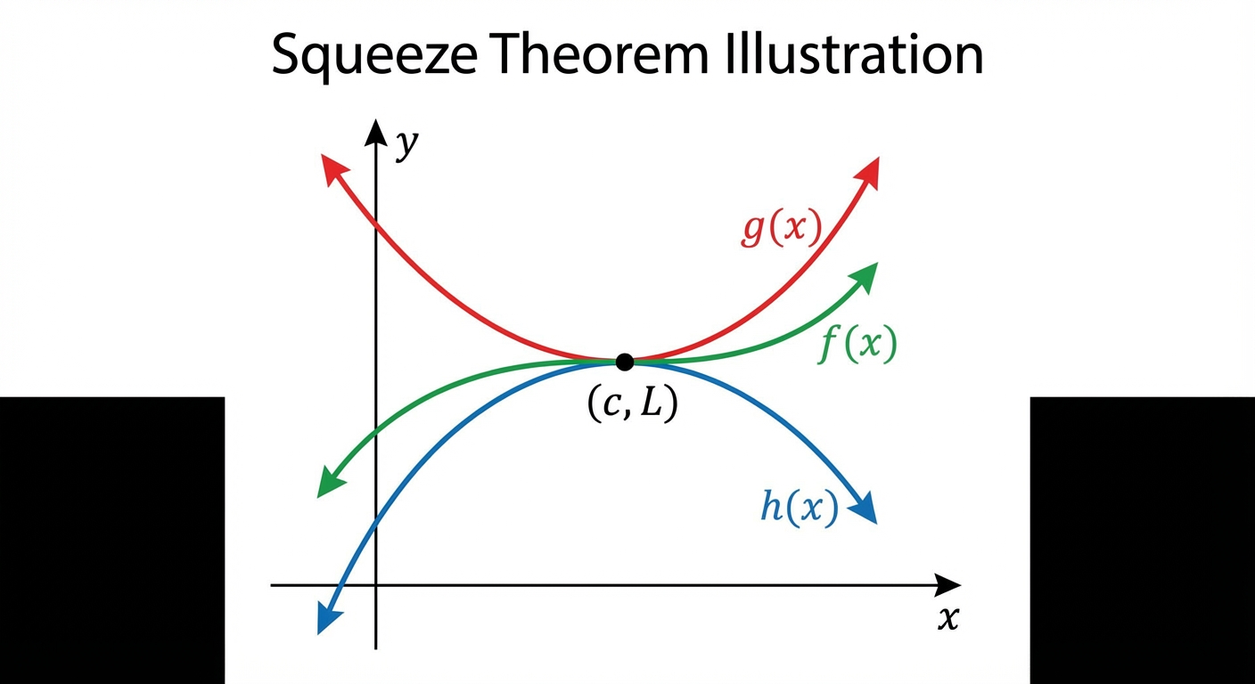
Squeeze theorem (Sandwich theorem)
The squeeze theorem is used when you can trap a complicated function between two simpler functions that approach the same limit.
If
for %%LATEX181%% near %%LATEX182%%, and
and
then
A good mental image: if %%LATEX186%% is squeezed into an ever-narrowing band and that band collapses to a single height %%LATEX187%%, then %%LATEX188%% must also approach %%LATEX189%%.
Common application: limits involving
or
which oscillate wildly.
Worked example: classic squeeze structure
Compute:
You might not be able to “simplify” . But you do know
Multiply the entire inequality by %%LATEX195%% (note %%LATEX196%% so inequality direction stays):
Now evaluate the bounding limits:
and
So the middle function is squeezed to :
Exam Focus
- Typical question patterns:
- Compute limits that initially give by factoring, rationalizing, or finding common denominators.
- Use trig limits (in radians), especially .
- Apply squeeze theorem when oscillation is bounded by functions with the same limit.
- Common mistakes:
- Canceling incorrectly (cancel factors only, not terms connected by addition/subtraction).
- Forgetting to use radians when applying trig limits.
- Using squeeze theorem without showing a valid inequality that holds near the point.
Infinite Limits and Limits at Infinity (Asymptotes and End Behavior)
Two different “infinity” ideas
Students often blend these together, but they are different:
- Infinite limit: what happens to %%LATEX204%% as %%LATEX205%% approaches a finite number (vertical asymptote behavior).
- Limit at infinity: what happens to %%LATEX207%% as %%LATEX208%% grows very large positive or very large negative (end behavior).
Infinite limits and vertical asymptotes
If as the function values increase without bound, you write
or if they decrease without bound,
This often corresponds to a vertical asymptote at .
A common trigger is: the denominator goes to 0 while the numerator does not.
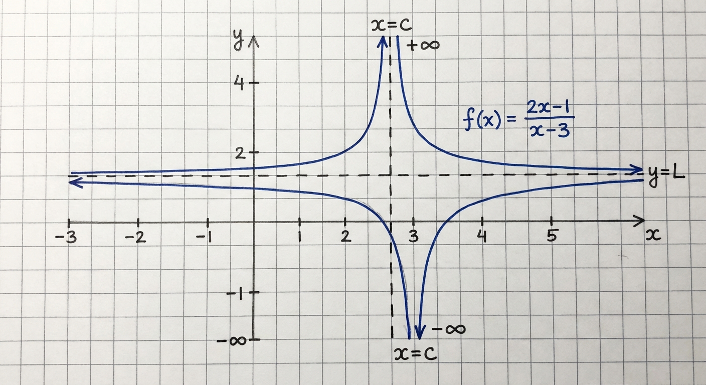
A classic rational example is
Then
and
Notice the one-sided limits differ in sign; the two-sided limit does not exist as a finite number.
Important AP language note: an “infinite limit” generally does not “exist” as a real number; you are describing unbounded behavior with %%LATEX216%% or %%LATEX217%%.
Worked example: one-sided infinite limits
Compute one-sided limits:
As , the denominator is a small positive number, so the fraction becomes very large positive:
For the left side:
As , the denominator is a small negative number, so the fraction becomes very large negative:
Limits at infinity and horizontal asymptotes
A limit at infinity asks about end behavior:
and
If the limit approaches a finite number %%LATEX226%%, then the graph has a horizontal asymptote %%LATEX227%% (as an end-behavior statement).
Rational functions: comparing degrees
For rational functions of the form
where %%LATEX229%% and %%LATEX230%% are polynomials, the end behavior is controlled by the highest-power terms.
Let %%LATEX231%% be the degree of %%LATEX232%% and %%LATEX233%% be the degree of %%LATEX234%%.
- If (bottom heavy), then
- If , then the limit at infinity is the ratio of leading coefficients.
- If %%LATEX238%% (top heavy), the function does not approach a finite horizontal asymptote; the limit at infinity diverges to %%LATEX239%% or does not exist as a finite number. Often there is a slant asymptote if the degree difference is exactly 1.
Worked example: degree numerator less than denominator
Compute:
As %%LATEX241%% becomes huge, %%LATEX242%% becomes huge, so the fraction approaches :
Additional bottom-heavy example
Compute:
The denominator grows faster than the numerator, so
Worked example: equal degrees
Compute:
The highest power is in both numerator and denominator, so the limit is the ratio of leading coefficients:
So the horizontal asymptote is .
Additional equal-degree example
Compute:
The degrees match, so the limit is the ratio of leading coefficients:
So the horizontal asymptote is .
Note on exponentials
Remember that grows faster than any polynomial. For example,
Why this matters for later calculus
End behavior and vertical asymptotes show up when you analyze derivatives and integrals too: you’ll eventually need to understand where a function “blows up,” where it levels off, and what its overall shape is.
Exam Focus
- Typical question patterns:
- Determine whether %%LATEX256%% is %%LATEX257%%, , or DNE using one-sided reasoning.
- Compute for rational functions by comparing degrees.
- Identify vertical and horizontal asymptotes from limit statements.
- Common mistakes:
- Treating as a number you can plug in (it describes unbounded behavior).
- Forgetting that one-sided behavior can differ at a vertical asymptote.
- Using leading-coefficient ratio when degrees are not equal.
- Writing arithmetic like “something over infinity.” Instead of treating infinity like a number, reason with end behavior (for instance, “dividing by a huge number approaches 0”).
Continuity: Connecting Limits to “No Breaks” Behavior
What continuity means (conceptually)
Continuity is one of the most frequently tested concepts on the AP exam. A function is continuous at a point if, near that point, the graph has no break, jump, or hole, and the function value matches the approaching value.
You can think of continuity as “the function behaves the way you expect substitution to work.” That’s why continuity is the bridge between limits and normal function evaluation.
Formal definition of continuity at a point (the 3-step test)
A function %%LATEX261%% is continuous at %%LATEX262%% if all three conditions hold:
- is defined.
- exists.
- .
Each condition matters:
- If %%LATEX266%% is not defined, you can’t have continuity at %%LATEX267%%.
- If the limit does not exist (jump or oscillation), you can’t have continuity.
- If the limit exists but does not equal (a misplaced point), you still don’t have continuity.
If a problem says “prove continuity,” you should explicitly address all three steps.
Continuity on an interval
- Continuous on an open interval means continuous at every point in the interval.
- On a closed interval %%LATEX269%%, continuity typically means continuous on %%LATEX270%% and also continuous from the right at %%LATEX271%% and from the left at %%LATEX272%%.
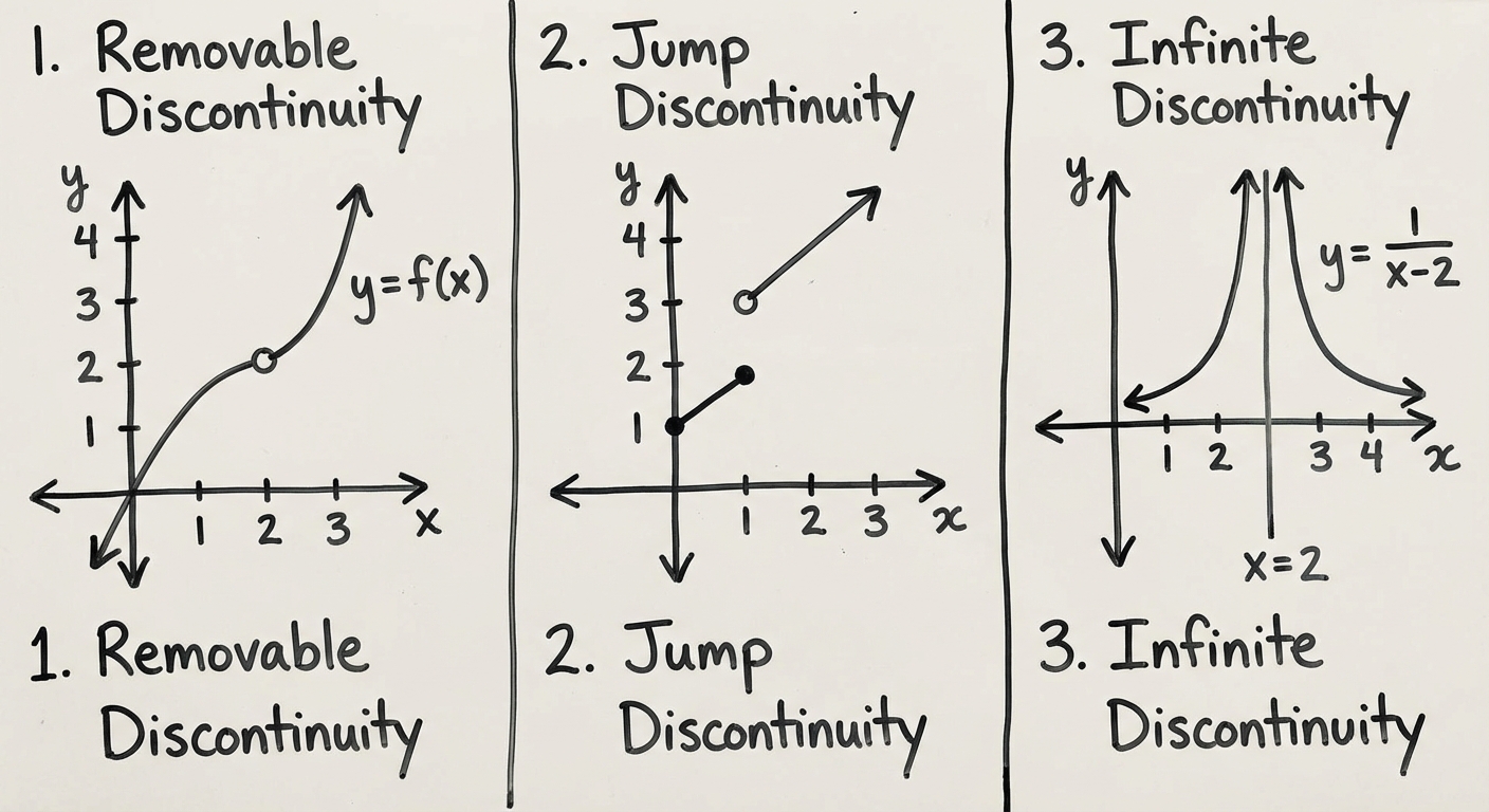
Types of discontinuities (what breaks continuity)
- Removable discontinuity (hole): The limit exists, but is missing or not equal to the limit. Algebraically, these often occur when factors cancel.
- Jump discontinuity: Left-hand and right-hand limits exist but are not equal. This is common in piecewise functions or step functions. A classic example structure is
- Infinite discontinuity (vertical asymptote): Function becomes unbounded near the point; one or both one-sided limits go to .
Example: checking continuity at a point
Suppose
Consider .
- %%LATEX278%% is not defined because the denominator becomes %%LATEX279%%.
- But you can simplify for :
So the limit exists:
The discontinuity is removable: the function is “missing” the value that would make it continuous.
Removing a discontinuity by redefining a value (extended function idea)
If you define a new function that matches the simplified expression for and then fill in the hole with the limit value, you create a function continuous at that point. This is sometimes described as forming an extended function.
Worked example: choosing a constant for continuity
A function is defined by
for %%LATEX285%%, and %%LATEX286%%. Find %%LATEX287%% so that %%LATEX288%% is continuous at .
Continuity requires
Factor and simplify (for ):
So
Continuity of common function types (practical facts)
In AP Calculus AB, you use these heavily:
- Polynomial functions are continuous for all real numbers.
- Rational functions are continuous wherever their denominators are not zero.
- Trigonometric functions like %%LATEX294%% and %%LATEX295%% are continuous for all real numbers.
These facts justify direct substitution quickly when allowed.
Exam Focus
- Typical question patterns:
- Determine whether a function is continuous at using the three conditions.
- Classify discontinuities as removable, jump, or infinite.
- Choose a constant (often called %%LATEX297%% or %%LATEX298%%) so a piecewise or modified function is continuous.
- “Prove continuity” prompts where you must explicitly show the 3-step test.
- Common mistakes:
- Claiming a function is continuous just because the limit exists (you also need defined and matching the limit).
- Mixing up removable and jump discontinuities (removable has matching one-sided limits).
- Forgetting to check the denominator for zero when asserting continuity of a rational function.
The Intermediate Value Theorem (IVT) and Why Continuity Has Power
The big promise of IVT
The Intermediate Value Theorem is an existence theorem: it guarantees a value exists, not where it is or what it equals exactly. It says that a continuous function on an interval can’t “skip” output values.
Informally: if the graph is unbroken and goes from below a certain y-value to above it, it must hit that y-value somewhere in between.
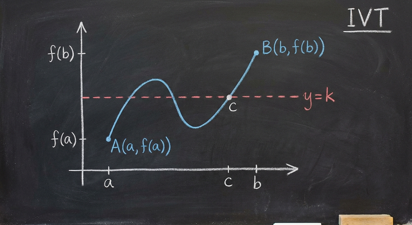
Formal statement
If %%LATEX300%% is continuous on %%LATEX301%% and %%LATEX302%% is any number between %%LATEX303%% and %%LATEX304%%, then there exists at least one number %%LATEX305%% in such that
A common special case is when you want to prove a root exists (a solution to %%LATEX308%%). If %%LATEX309%% and %%LATEX310%% have opposite signs and %%LATEX311%% is continuous on %%LATEX312%%, then there is at least one %%LATEX313%% in with
Many textbook and exam statements use %%LATEX316%% in the open interval %%LATEX317%%, but the key idea is: the guaranteed point lies somewhere between the endpoints.
Why IVT matters in calculus and applications
IVT is a guarantee of existence, not a method for finding the exact value. This is powerful in real life:
- In physics, if a continuous position function changes from one side of a point to the other, the object must pass through that point.
- In engineering, if a continuous error function changes sign over time, there is a time when the error is exactly zero.
- In numerical methods, IVT is the logic behind bracketing methods (like bisection) for locating roots.
Real world analogy: If you were 3 feet tall at age 5 and 5 feet tall at age 12, there must have been a moment when you were exactly 4 feet tall (assuming growth is continuous).
What IVT does not tell you
IVT does not tell you:
- how many solutions there are
- what the exact solution is
- that the function is one-to-one
It only guarantees at least one solution exists.
Worked example: using IVT to prove a root exists
Let
Show that %%LATEX319%% has a solution between %%LATEX320%% and .
- Check continuity: %%LATEX322%% is a polynomial, so it is continuous on all real numbers, including %%LATEX323%%.
- Compute endpoint values:
- Since %%LATEX326%% is negative and %%LATEX327%% is positive, %%LATEX328%% lies between %%LATEX329%% and .
By IVT, there exists at least one %%LATEX331%% in %%LATEX332%% such that
Worked example: IVT for a nonzero target value
Suppose %%LATEX334%% is continuous on %%LATEX335%% with %%LATEX336%% and %%LATEX337%%. Then for any number %%LATEX338%% between %%LATEX339%% and %%LATEX340%% (like %%LATEX341%%), there exists %%LATEX342%% in %%LATEX343%% such that
This is exactly the “can’t skip values” idea.
Typical exam problem: show a zero exists on an interval
Show that
has a zero on the interval .
- Continuity: %%LATEX347%% is a polynomial, so it is continuous on %%LATEX348%%.
- Compute endpoints:
- Since
by IVT there exists a %%LATEX352%% in %%LATEX353%% such that
Exam Focus
- Typical question patterns:
- Use IVT to justify that an equation has a solution in an interval.
- Identify the correct interval where a root must exist by checking sign changes.
- Explain why continuity is necessary for the conclusion.
- Common mistakes:
- Using IVT without first stating that %%LATEX356%% is continuous on %%LATEX357%%.
- Claiming IVT gives the exact value of the solution (it only guarantees existence).
- Forgetting that the target output must be between %%LATEX358%% and %%LATEX359%% (order doesn’t matter, but “between” does).
Common Mistakes & Pitfalls (Unit 1)
Students lose a lot of points in Unit 1 for small logic and notation errors. These are the big ones to watch for.
- The “0/0” answer: Never write as a final answer. It is an instruction to do more work (factor, conjugate, common denominators, trig identities, etc.).
- Confusing limit value vs. function value: A limit can exist even if the function is undefined at that point (a hole). Limits describe approaching behavior, not the value at the point.
- Mismatched notation in one-sided limits: The superscript minus in means “from the left,” not “to negative 2.”
- Forgetting conditions for IVT: You cannot apply IVT unless you state that the function is continuous on the interval.
- Substituting infinity: Infinity is not a number. Do not do arithmetic “plugging in infinity.” Instead, reason with growth rates and end behavior.
Exam Focus
- Typical question patterns:
- “Explain why” free-response justifications: graders look for the correct vocabulary (continuous, one-sided limits match, sign change, etc.).
- Notation accuracy checks: correctly distinguishing %%LATEX362%%, %%LATEX363%%, and .
- Common mistakes:
- Writing a conclusion (like “by IVT there is a root”) without stating the needed hypothesis (continuity on the closed interval).
- Treating like a normal value you can substitute into expressions.