Unit 4: Market Structures of Imperfect Competition
Introduction to Monopoly
A Monopoly represents a market structure at the opposite end of the spectrum from Perfect Competition. In this structure, a single firm dictates the market conditions. Understanding the monopoly is crucial because it introduces the concept of the Price Maker—a firm that must lower its price to sell more units, fundamentally changing how revenue is calculated compared to perfect competition.
Key Characteristics of Monopoly
To identify a monopoly, look for these four specific conditions:
- Single Seller: One firm controls the entire industry. The firm is the industry.
- Unique Product: There are no close substitutes for the good or service.
- High Barriers to Entry: Extremely difficult for new firms to enter the market due to geography, government mandates (patents), or technology.
- Price Maker: The firm has significant control over the price it charges.
The Relationship Between Demand and Marginal Revenue
Unlike a perfectly competitive firm where Price equals Marginal Revenue ($P = MR$), a monopoly faces a downward-sloping market demand curve. To sell an additional unit, the monopolist must lower the price not just for that new unit, but for all previous units.
Consequently, the Marginal Revenue (MR) curve lies below the Demand (D) curve.

Revenue Formulas
- Total Revenue (TR):
- Average Revenue (AR):
- Marginal Revenue (MR):
Visual Tip: The MR curve generally starts at the same point on the Y-axis as the Demand curve but has twice the slope (it is steeper).
Profit Maximization
Just like every other firm in economics, monopolists follow the Golden Rule of Profit Maximization:
Steps to identify price and quantity on a graph:
- Find the intersection where the MR curve hits the MC curve.
- Go down to the X-axis to find the profit-maximizing quantity ($Q_m$).
- Go up from that quantity to the Demand Curve (not the MR curve!) and across to the Y-axis to find the price ($P_m$).
Elasticity and Revenue
A monopoly will only produce in the elastic range of the demand curve. Why?
- Elastic Range: When price lowers, TR increases ($MR > 0$).
- Unit Elastic: TR is maximized ($MR = 0$).
- Inelastic Range: When price lowers, TR decreases ($MR < 0$). Since MC is always positive, a firm would never produce where MR is negative.
Efficiency and Regulation
Monopolies are considered market failures because they are inefficient compared to perfect competition.
Types of Inefficiency
- Allocatively Inefficient: The firm produces less than society wants. Price is greater than Marginal Cost ($P > MC$). This results in Deadweight Loss (DWL).
- Productively Inefficient: The firm does not produce at the lowest possible cost. Price is greater than the minimum Average Total Cost ($P > min\ ATC$).
Natural Monopolies
A Natural Monopoly occurs when economies of scale are so extensive that one firm can supply the entire market at a lower average cost than two or more firms could. This is common in utilities (e.g., electricity, water).

Regulation Policy Options
Governments often regulate natural monopolies to protect consumers. There are two common price ceilings:
- Socially Optimal Price ($P = MC$): This achieves allocative efficiency but forces the firm to incur a loss (requires a subsidy to stay in business).
- Fair Return Price ($P = ATC$): The firm breaks even (Normal Profit). It is not allocatively efficient, but the firm survives without subsidies.
Price Discrimination
Price Discrimination involves selling the same product to different buyers at different prices based on their willingness to pay, rather than cost differences.
Conditions for Price Discrimination
- The firm must have monopoly power (market power).
- The firm must be able to segregate the market (identify distinct groups).
- Consumers must not be able to resell the product (no arbitrage).
Perfect (First-Degree) Price Discrimination
If a monopoly can charge exactly what each consumer is willing to pay:
- The Demand curve becomes the Marginal Revenue curve ($D = MR$).
- Consumer Surplus is 0 (it is all converted into profit/producer surplus).
- Deadweight Loss is 0 (the firm produces the allocatively efficient quantity).
Monopolistic Competition
Monopolistic Competition is a "hybrid" market structure combining elements of Perfect Competition and Monopoly. Think of fast food, clothing brands, or hair salons.
Key Characteristics
- Many Sellers: Hundreds of firms.
- Differentiated Products: Products are similar but not identical (branding, quality, location).
- Low Barriers to Entry/Exit: Easy for firms to start or stop business.
- Some Control over Price: They are price makers, but demand is highly elastic due to substitutes.
Short-Run vs. Long-Run Equilibrium
In the Short Run:
A monopolistically competitive firm looks exactly like a monopoly graph. It can make positive economic profit or incur a loss.
In the Long Run:
Because entry is easy, economic profits cannot exist in the long run.
- If Profits exist: New firms enter $\rightarrow$ More substitutes $\rightarrow$ Firm's Demand shifts Left $\rightarrow$ Price falls $\rightarrow$ Zero Economic Profit.
- If Losses exist: Firms exit $\rightarrow$ Fewer substitutes $\rightarrow$ Firm's Demand shifts Right $\rightarrow$ Price rises $\rightarrow$ Zero Economic Profit.
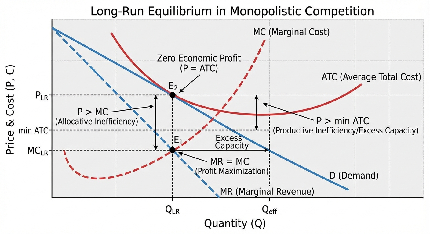
Excess Capacity
In the long run, the firm produces where $MR = MC$, but the price is set where the Demand curve is tangent to the ATC curve. This point is to the left of the minimum ATC.
- Excess Capacity Definition: The gap between the actual output produced and the output required to minimize ATC (productive efficiency).
- These firms have the capacity to produce more at a lower average cost, but they choose not to in order to maintain a higher price.
Common Mistakes & Pitfalls
1. Confusing "High Price" with "Highest Price"
- Mistake: Students often assume monopolists charge the highest possible price.
- Correction: Monopolists charge the profit-maximizing price ($MR=MC$), not the highest price. Charging too high reduces quantity demanded so much that total profit falls.
2. The Supply Curve Fallacy
- Mistake: Drawing a supply curve for a monopoly.
- Correction: Monopolies do not have a supply curve. There is no one-to-one relationship between price and quantity supplied because the firm sets both based on demand.
3. Allocative Efficiency in Monopolistic Competition
- Mistake: Thinking that zero economic profit in the long run means the market is efficient.
- Correction: Even in the long run with zero profit, monopolistic competition is inefficient. Price is still greater than Marginal Cost ($P > MC$), leading to Deadweight Loss.
4. Revenue Max vs. Profit Max
- Mistake: Confusing Revenue Maximization with Profit Maximization.
- Correction:
- Profit Max: $MR = MC$
- Revenue Max: $MR = 0$ (This is usually a higher quantity and lower price than the profit-max point).