AP Calculus AB Unit 7 Study Guide: Differential Equations (Slope Fields, Separable IVPs, Euler’s Method, Exponential & Logistic Models)
What Differential Equations Are and How They Model Change
A differential equation is an equation that relates an unknown function (often written as %%LATEX0%% as a function of %%LATEX1%%) to one or more of its derivatives (like ). In plain language: instead of telling you the function directly, it tells you how the function changes.
This connects nicely to ideas you’ve already seen in related rates: in both topics, the main object is a rate of change (a derivative). The difference is that in differential equations, you’re often using a rule about rates to reconstruct the original function.
That idea matters because many real-world situations are naturally described by change rules rather than explicit formulas. For example:
- A population might grow at a rate proportional to its current size.
- The amount of medicine in your bloodstream might decrease at a rate proportional to how much is present.
- The temperature of coffee might cool at a rate proportional to the difference between the coffee’s temperature and room temperature.
In each case, you often know (or assume) a rule for the rate of change, and you want to find the function itself.
Differential equation vs. explicit function
In earlier units, you often started with a function %%LATEX3%% and then found %%LATEX4%%. Differential equations reverse the direction:
- You start with something like .
- You use calculus (integration, plus algebra) to work back to .
A key point: a differential equation typically has infinitely many solutions, a whole family of functions, because differentiation “loses information” (constants disappear). To pick one specific solution, you need an initial condition.
Notation you must recognize
Differential equations appear in several equivalent notations. You’re expected to translate among them fluently.
| Meaning | Common notations |
|---|---|
| Derivative of %%LATEX7%% with respect to %%LATEX8%% | %%LATEX9%%, %%LATEX10%% |
| Differential equation giving slope | |
| Second derivative | %%LATEX12%%, %%LATEX13%% |
You’ll see both %%LATEX14%% and %%LATEX15%% on AP-style questions.
Solution, general solution, particular solution
A solution to a differential equation is a function %%LATEX16%% that makes the equation true when you substitute %%LATEX17%% and its derivative(s).
A general solution describes a family of solutions using an arbitrary constant %%LATEX18%%. A particular solution is the one function you get after using an initial condition to find %%LATEX19%%.
For example, if solving leads to
that’s a general solution. If you also know %%LATEX21%%, then %%LATEX22%% so and the particular solution is
Checking a proposed solution (a skill that shows up often)
To verify that a function solves a differential equation:
- Compute the derivative(s) required by the differential equation.
- Substitute the function and its derivative(s) into the differential equation.
- Confirm both sides match for all in the domain.
This is conceptually simple but easy to mess up with derivative errors.
Example: verify a solution
Check whether
solves
Compute derivative:
Right-hand side:
They match, so is a solution.
Exam Focus
- Typical question patterns:
- “Show that the function %%LATEX31%% satisfies the differential equation %%LATEX32%%.”
- “Write a differential equation that models the situation described (rate proportional to…, limited by carrying capacity, etc.).”
- “Find the particular solution given an initial condition.”
- Common mistakes:
- Forgetting that solutions are functions: plugging in a single point instead of substituting the whole function.
- Mixing up %%LATEX33%% and %%LATEX34%% (for example, substituting %%LATEX35%% where %%LATEX36%% belongs).
- Differentiation slips when verifying (especially chain rule with exponentials).
Slope Fields (Direction Fields) and Qualitative Solutions
A slope field (also called a direction field) is a picture that shows the slope %%LATEX37%% at many points (x, y) without explicitly solving the differential equation. At each point, you draw a small line segment with slope equal to the value of %%LATEX38%% in
This matters because many differential equations are hard (or impossible in a typical AP setting) to solve symbolically, but you can still understand behavior: where solutions increase or decrease, where they level off, and how initial conditions change the resulting curve.
How to construct a slope field (plug-and-draw)
To construct a slope field, you plug in the coordinates (the x-value, the y-value, or both, depending on the differential equation) into the right-hand side and sketch a short segment with that slope.
For example, for
the slope at any point with %%LATEX41%% is %%LATEX42%% (because the slope depends only on ).
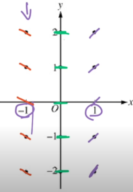
How to read a slope field
When you look at the small segments:
- Segments slanting upward mean so solution curves increase.
- Segments slanting downward mean so solution curves decrease.
- Horizontal segments mean so solution curves have a horizontal tangent there.
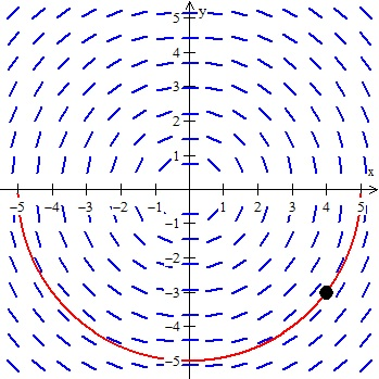
A solution curve is a smooth curve that is always tangent to the tiny segments. You can sketch one solution by “following the flow” of the field.
The AP exam might require you to sketch a solution curve given a slope field. The key is to “flow” with the slopes: your curve should look like it is made of tangent pieces aligned with the little segments. Because this is done by hand, it doesn’t have to be exact, but it should not cross the direction segments abruptly.
Isoclines (where slopes are equal)
An isocline is a curve in the xy-plane along which the slope field has the same slope value. If
then the set of points satisfying %%LATEX48%% is an isocline for slope %%LATEX49%%. Isoclines help you organize slope fields: find where slope is %%LATEX50%%, where slope is %%LATEX51%%, etc.
Equilibrium (constant) solutions
An equilibrium solution (also called a constant solution) is a solution where %%LATEX52%% stays constant as %%LATEX53%% changes, meaning
If the differential equation is autonomous (depends only on ), like
then equilibria occur at values of %%LATEX57%% where %%LATEX58%%. On a slope field, these show up as horizontal segments across an entire horizontal line.
Equilibria matter because they often represent long-term behavior: populations stabilizing, temperatures approaching room temperature, and so on.
Stability (qualitative)
If you have an autonomous differential equation %%LATEX59%% and an equilibrium at %%LATEX60%%:
- The equilibrium is stable if solution curves near %%LATEX61%% move toward %%LATEX62%% over time.
- It is unstable if nearby solutions move away.
You can often tell from the sign of %%LATEX63%% above and below %%LATEX64%%:
- If %%LATEX65%% just below %%LATEX66%% (solutions increase) and %%LATEX67%% just above %%LATEX68%% (solutions decrease), then solutions are pushed toward : stable.
- Reverse signs imply unstable.
Example: stability from signs
Suppose
Equilibria: solve %%LATEX71%% giving %%LATEX72%% and .
Test intervals:
- If %%LATEX74%%, then %%LATEX75%% and %%LATEX76%% so %%LATEX77%%: solutions increase.
- If %%LATEX78%%, then %%LATEX79%% so : solutions decrease.
So solutions move toward %%LATEX81%% from both sides: %%LATEX82%% is stable. Near %%LATEX83%%, if %%LATEX84%% then %%LATEX85%% so solutions decrease (move away from %%LATEX86%%), and if %%LATEX87%% they increase (also away from %%LATEX88%%), so is unstable.
Exam Focus
- Typical question patterns:
- “Sketch the slope field for and sketch the solution curve through a given initial point.”
- “Use the slope field to estimate %%LATEX91%% given %%LATEX92%%.”
- “Identify equilibrium solutions and classify stability from a direction field or from the sign of .”
- Common mistakes:
- Drawing solution curves that cross direction segments instead of staying tangent.
- Treating the slope as depending only on %%LATEX94%% or only on %%LATEX95%% when it depends on both.
- Confusing an isocline (same slope) with a solution curve (a specific integral curve).
- Forgetting that a slope field is built by plugging points into the differential equation (for example, for %%LATEX96%%, all points with the same %%LATEX97%% share the same slope).
Initial Value Problems (IVPs) and Particular Solutions
An initial value problem (IVP) is a differential equation together with an initial condition that specifies the value of the solution at a particular input.
A typical IVP looks like:
The initial condition is what selects one unique member from the family of solutions.
Why IVPs matter
In applications, you almost always know some starting measurement: the initial population, initial temperature, initial amount of a drug, initial position, etc. The differential equation gives a general rule of change, but the initial condition pins down the actual situation.
Existence and uniqueness (conceptual)
In AP Calculus AB, you’re generally expected to know the idea that under reasonable conditions (specifically when %%LATEX100%% and its partial derivative with respect to %%LATEX101%% are continuous near the initial point), an IVP has a unique solution through that point. Practically:
- A well-behaved slope field should show exactly one solution curve passing through the initial point.
If a slope field shows multiple curves that could pass through the same point (or a cusp/vertical tangent situation where the differential equation isn’t defined nicely), uniqueness can fail.
Using initial conditions after solving
A very common workflow:
- Solve the differential equation to get a general solution with a constant .
- Plug the initial condition into the general solution to find .
- Write the particular solution.
Example: particular solution from an IVP
Solve the IVP:
Step 1: integrate both sides with respect to :
Step 2: use the initial condition :
So the particular solution is:
A subtle but important habit: when you integrate, always include (or you will lose the ability to satisfy the initial condition).
Exam Focus
- Typical question patterns:
- “Find the particular solution to the differential equation that satisfies .”
- “Given a slope field and a point, sketch the solution and estimate a value.”
- “Determine whether the solution is increasing/decreasing at a point using the differential equation.”
- Common mistakes:
- Forgetting the constant of integration, then being unable to match the initial condition.
- Plugging the initial condition into the differential equation instead of into the solved function.
- Mixing up the meaning of (it means the point (a, b) lies on the solution curve).
Euler’s Method: Approximating Solutions Numerically
Often you cannot (or are not asked to) solve a differential equation explicitly. Euler’s method is a numerical technique that approximates the solution to an IVP by using tangent line steps.
Suppose you have:
and an initial condition .
Euler’s method uses the idea: near %%LATEX119%%, the solution curve looks like its tangent line. The slope at (x0, y0) is %%LATEX120%%, so if you take a small step of size %%LATEX121%% in %%LATEX122%%, the change in is approximately slope times run:
So the next approximate point is:
Then you repeat: compute the slope at (x1, y1), step again, and so on.
The Euler update formulas
If you label the approximate points , then:
Here:
- %%LATEX130%% is the step size (for example, %%LATEX131%% or ).
- Smaller usually gives better accuracy but requires more steps.
Why Euler’s method makes sense (conceptually)
Euler’s method is repeated local linearization. Every step uses a tangent line approximation. It’s the same idea as using the linearization formula from derivatives:
but with %%LATEX135%% replaced by %%LATEX136%% because the slope depends on both variables.
Error behavior (what you should know)
Euler’s method can accumulate error because:
- Each step uses an approximation.
- If the approximation is slightly off, the next slope calculation is based on a slightly wrong point.
You should still expect these truths:
- Decreasing tends to improve the approximation.
- Over many steps, errors can grow.
AP questions often test whether you can execute the algorithm accurately and interpret what the approximation means.
Example: Euler’s method computation
Approximate for the IVP:
Use step size .
Start: %%LATEX142%%, %%LATEX143%%.
Step to :
Slope at (0, 1):
Update:
Step to :
Slope at (0.1, 1.1):
Update:
Step to :
Slope at (0.2, 1.22):
Update:
So Euler’s method gives
A common interpretation point: this number is not exact; it is an approximation produced by three tangent-line steps.
Exam Focus
- Typical question patterns:
- “Use Euler’s method with step size %%LATEX154%% to approximate %%LATEX155%% at a given value.”
- “Set up a table of values for Euler’s method and fill in the missing entries.”
- “Compare two Euler approximations with different step sizes and decide which should be more accurate.”
- Common mistakes:
- Using the wrong point when computing slope (mixing %%LATEX157%% with %%LATEX158%%).
- Forgetting to multiply by step size .
- Rounding too early and compounding error; keep several decimals until the end unless instructed otherwise.
Separable Differential Equations: Solving by Separating Variables
A separable differential equation is one where you can algebraically rearrange the equation so that all %%LATEX160%%-terms are on one side and all %%LATEX161%%-terms are on the other. This is the main symbolic solving technique emphasized in AP Calculus AB for differential equations.
The general form you’re aiming for is:
Then you “separate”:
and integrate both sides.
Why separation works
At a conceptual level, separating variables is leveraging the fact that integration “undoes” differentiation. If you can express the derivative as a product of an %%LATEX164%%-only part and a %%LATEX165%%-only part, then you can integrate each side with respect to its own variable.
A frequent point of confusion is the notation. When you write
you can treat it like a fraction for the purpose of rearranging:
and then multiply both sides by :
This is a standard technique in AP Calculus, even though in more advanced math courses you learn a more rigorous justification.
The general solving process (with key habits)
A reliable checklist is:
- Separate variables so that the left side involves only %%LATEX170%% and %%LATEX171%%, and the right side involves only %%LATEX172%% and %%LATEX173%%.
- Integrate both sides.
- Add a constant of integration (usually just on one side).
- Solve for if possible (sometimes leaving an implicit solution is acceptable).
- Apply initial conditions to find the constant and get a particular solution.
A helpful memory trick for these problems is SIPPY:
- S: Separate (put %%LATEX175%% and %%LATEX176%% on separate sides)
- I: Integrate (remove the derivative)
- P: Plus C (include the constant)
- P: Plug in your initial condition
- Y: Y equals (solve to isolate , if possible)
Two habits prevent many errors:
- Make sure you integrate with respect to the correct variable.
- Do not drop absolute values when integrating .
Example 1: basic separation
Solve:
Step 1: separate:
Step 2: integrate:
Step 3: solve for by exponentiating:
Rewrite %%LATEX185%% as a new constant %%LATEX186%%:
This means %%LATEX188%% could be positive or negative; you can absorb the sign into a nonzero constant %%LATEX189%%:
That is the general solution.
Example 2: separation with an initial condition
Solve the IVP:
Separate:
Integrate:
Exponentiate:
Use :
So and the particular solution is:
Example 3: separable IVP from the SIPPY checklist
Solve:
with
Separate by multiplying both sides by :
Integrate both sides:
Plus C is essential here.
Plug in the initial condition :
So
Now Y equals: first rewrite the equation, then solve for .
Multiply both sides by 2:
Take the square root:
Since is positive, we choose the positive branch:
Implicit solutions are sometimes the natural stopping point
Not every separable differential equation solves neatly for . For example, you might end with something like
That is still a valid solution description. On AP-style tasks, if the question asks you to “solve” without specifying explicit form, an implicit solution is often acceptable.
Exam Focus
- Typical question patterns:
- “Solve the differential equation by separation of variables.”
- “Find the particular solution that satisfies .”
- “Show that a given function is a solution by substituting into the differential equation.”
- Common mistakes:
- Separating incorrectly (for example, leaving an %%LATEX217%% on the %%LATEX218%% side).
- Forgetting absolute value in %%LATEX219%% after integrating %%LATEX220%%.
- Losing constant solutions (equilibria) by dividing by an expression that could be zero (for example, dividing by %%LATEX221%% without noting %%LATEX222%% may be a solution).
- Forgetting the “Plus C” step, which prevents you from fitting an initial condition.
Differential Equations as Models: Setting Up Equations From Words
A big part of Unit 7 is translating a description of a changing quantity into a differential equation. In modeling, the derivative represents a rate with units that tell you what the derivative means.
If %%LATEX223%% is a quantity (population, mass, temperature) and %%LATEX224%% is time, then
means “rate of change of %%LATEX226%% per unit time.” If %%LATEX227%% is measured in people and %%LATEX228%% in days, then %%LATEX229%% has units people per day.
Proportionality models
The phrase “proportional to” is a huge clue. If a rate is proportional to a quantity, you typically write:
where is the constant of proportionality.
If it’s proportional to the difference between a quantity and some baseline , you often write:
The sign of %%LATEX234%% determines whether the quantity moves toward or away from %%LATEX235%%.
Interpreting parameter meanings
In a model like
- %%LATEX237%% means growth (the larger %%LATEX238%% is, the faster it increases).
- %%LATEX239%% means decay (the larger %%LATEX240%% is, the faster it decreases).
In models like logistic growth, parameters have concrete interpretations (carrying capacity, growth rate), and AP problems may ask what those parameters mean in context.
Example: build a differential equation
“A bacteria culture grows at a rate proportional to the number of bacteria present.”
Let %%LATEX241%% be the number of bacteria at time %%LATEX242%%. “Rate proportional to the amount present” translates to:
If it additionally says “it doubles every 3 hours,” that would be used later to solve for after solving the differential equation.
Example: rate depends on both time and amount
If the statement gives a rate explicitly as a function of both variables, you write it directly. For instance:
“The rate of change of %%LATEX245%% is given by %%LATEX246%%.”
That already is the differential equation. Your job might then be slope field analysis or numerical approximation rather than symbolic solution.
Exam Focus
- Typical question patterns:
- “Write a differential equation that models the situation described.”
- “Identify what the constant represents and determine its sign.”
- “Use units to interpret and to check whether a model makes sense.”
- Common mistakes:
- Confusing proportional to %%LATEX249%% with proportional to %%LATEX250%% (reading too quickly and assigning the wrong variables).
- Choosing the wrong sign for decay or cooling situations.
- Ignoring units, which often reveal an incorrect setup.
Exponential Growth and Decay as Differential Equations
Exponential growth and decay are among the most important applications of differential equations because they arise from one simple assumption:
The rate of change of a quantity is proportional to the amount of that quantity present.
Mathematically, if %%LATEX251%% is the quantity and %%LATEX252%% is time:
Solving the exponential differential equation
This is separable:
Integrate:
Exponentiate:
Here %%LATEX257%% is a nonzero constant. If you are modeling a quantity like population, you typically take %%LATEX258%%.
If an initial condition is given, such as , then:
So and the solution becomes:
Connecting to familiar exponential forms
You may also be familiar with discrete forms like %%LATEX263%%. The differential equation model naturally leads to the base-%%LATEX264%% form %%LATEX265%%. They describe the same kind of behavior, with %%LATEX266%% acting as a continuous growth rate.
Doubling time and half-life
If a quantity grows exponentially, the doubling time is constant (it does not depend on the current amount). If a quantity decays exponentially, the half-life is constant.
Using :
Doubling means , so
Half-life means , so
Since decay has , this yields a positive half-life.
Example: find from doubling time
A population satisfies %%LATEX278%% and doubles in 5 years. Find %%LATEX279%%.
From the general solution:
Doubling in 5 years means :
Example: decay with half-life
A substance decays according to %%LATEX286%%. Its half-life is 12 days. Express %%LATEX287%%.
Half-life condition: .
This is negative, consistent with decay.
A common conceptual trap: “rate proportional to amount” implies exponential, not linear
Students sometimes think “constant rate” and “proportional rate” are the same. They’re not:
- If %%LATEX294%% (constant), the solution is linear: %%LATEX295%%.
- If %%LATEX296%% (proportional to amount), the solution is exponential: %%LATEX297%%.
In words: constant rate means you add the same amount each time step; proportional rate means you multiply by the same factor over equal time intervals.
Exam Focus
- Typical question patterns:
- “Given %%LATEX298%% and a condition like doubling time or half-life, find %%LATEX299%% and the function .”
- “Interpret the meaning of (growth vs. decay) in context.”
- “Use the solution to compute a time when the quantity reaches a given value.”
- Common mistakes:
- Solving for %%LATEX302%% but forgetting to use the time value (for example, using %%LATEX303%% instead of ).
- Forgetting that decay requires %%LATEX305%%; if you get %%LATEX306%% for a decay context, re-check your algebra.
- Dropping absolute value too early when integrating (less common in pure application problems, but it appears in derivations).
Logistic Growth: Growth With a Carrying Capacity
Exponential growth assumes unlimited resources. Many real populations cannot grow forever at a rate proportional to their size because resources become limiting. Logistic growth modifies exponential growth by introducing a maximum sustainable population, called the carrying capacity.
A common logistic differential equation is:
Where:
- %%LATEX309%% is the population at time %%LATEX310%%.
- is a positive growth constant (related to how quickly the population grows when small).
- is the carrying capacity.
Why this model behaves differently than exponential growth
Look at the factor:
- If %%LATEX314%% is small compared to %%LATEX315%%, then %%LATEX316%% is near 0, so the factor is near 1. The equation behaves like exponential growth %%LATEX317%%.
- If %%LATEX318%% approaches %%LATEX319%%, then approaches 0, so growth slows down.
- If %%LATEX321%%, then %%LATEX322%% is negative, making %%LATEX323%%, so the population decreases back toward %%LATEX324%%.
So acts like a “target level” that solutions tend to approach.
Equilibria and stability in logistic growth
Equilibria occur when . For logistic:
So equilibria are:
Qualitatively:
- is typically stable.
- %%LATEX331%% is unstable (if %%LATEX332%% is slightly above 0, it tends to increase).
The logistic equation is separable
You can solve it explicitly by separation of variables. Start with:
Rewrite the right side:
Separate:
At this point, the left side requires partial fractions to integrate. On AP Calculus AB, you are sometimes given the solved form, or you may be asked to work with the differential equation qualitatively or numerically rather than doing the full algebra. Still, it’s important to know what the explicit solution looks like and how to interpret it.
A standard explicit form is:
where is determined from the initial condition.
Finding the constant from an initial condition
If , then
Solve for :
So the particular solution can be written:
Interpreting logistic solution features
A logistic solution has an S-shape when %%LATEX344%% is between 0 and %%LATEX345%%:
- Early on, it grows almost exponentially.
- Then growth speeds up until an inflection point.
- After that, growth slows and levels off near .
The growth rate is maximized at
This can be shown by treating %%LATEX349%% as a function of %%LATEX350%% and finding its maximum.
Example: qualitative logistic reasoning without full solving
Given
- If %%LATEX352%%, then %%LATEX353%%, so %%LATEX354%% and relatively close to %%LATEX355%%.
- If %%LATEX356%%, then %%LATEX357%%, so is still positive but much smaller: growth is slow.
- If %%LATEX359%%, then %%LATEX360%%, so : the population decreases.
This kind of sign-and-magnitude reasoning is common on free-response questions.
Exam Focus
- Typical question patterns:
- “A population is modeled by a logistic differential equation. Identify the carrying capacity and interpret what it means.”
- “Use the differential equation to determine whether the population is increasing or decreasing at a given value of .”
- “Given the explicit logistic solution, use an initial condition to find the constant and compute values.”
- Common mistakes:
- Treating logistic growth as exponential and forgetting the limiting factor .
- Misidentifying carrying capacity: it is the value of %%LATEX364%% where the derivative becomes 0 in a stable way (usually %%LATEX365%%).
- Algebra errors solving for %%LATEX366%% from %%LATEX367%% (especially forgetting that ).
Using Differential Equations to Analyze Behavior Without Solving Exactly
One of the most powerful ideas in this unit is that you can answer many questions without finding an explicit formula for . The differential equation itself tells you slopes, increasing/decreasing behavior, concavity (sometimes), and long-term trends.
Increasing and decreasing from the sign of the derivative
If you know
then at a point (x, y) on a solution:
- If , the solution is increasing there.
- If , the solution is decreasing there.
This is the same logic as derivative sign analysis for ordinary functions, except now the derivative is given in terms of both variables.
Horizontal tangents and equilibrium levels
Horizontal tangent means:
So you can find where solutions might level off by solving %%LATEX374%% (or %%LATEX375%% in autonomous cases). In modeling, those often represent steady states.
Concavity from differentiating the differential equation
Sometimes you’re asked about concavity of the solution curve even when you don’t know %%LATEX376%% explicitly. You can find %%LATEX377%% by differentiating both sides with respect to .
If
then
Because %%LATEX381%% depends on %%LATEX382%% and %%LATEX383%%, this derivative often requires the chain rule: when differentiating with respect to %%LATEX384%%, treat %%LATEX385%% as a function of %%LATEX386%%.
Example: concavity from a differential equation
Suppose
Differentiate both sides with respect to :
The derivative of %%LATEX390%% is 1. The derivative of %%LATEX391%% with respect to %%LATEX392%% is %%LATEX393%%. So:
Now substitute the original expression for :
So at any point (x, y) on a solution curve, concavity depends on whether is positive (concave up) or negative (concave down).
A common mistake here is to treat %%LATEX398%% as a constant when differentiating. In this context, %%LATEX399%% changes with .
Long-term behavior in autonomous equations
For autonomous equations
you can often predict long-term behavior by looking at equilibria and sign charts. This is especially common with logistic-type models.
Exam Focus
- Typical question patterns:
- “Given , determine whether the solution through a point is increasing/decreasing (and sometimes concave up/down).”
- “Find where solutions have horizontal tangents by solving .”
- “Use an autonomous differential equation to determine limiting behavior as increases.”
- Common mistakes:
- Confusing the point (x, y) with the initial condition and assuming it holds for all .
- Differentiating %%LATEX406%% incorrectly when finding %%LATEX407%% (forgetting appears via chain rule).
- Treating equilibrium solutions as just “points” rather than full constant functions .
Differential Equations in Motion Contexts (Position, Velocity, Acceleration)
Motion is a natural place where derivatives appear:
- Position
- Velocity
- Acceleration
A differential equation might relate these quantities. For example, if acceleration depends on velocity, you may get a differential equation for .
Why motion problems connect well to Unit 7
You’ve already learned that integrating velocity gives displacement and integrating acceleration gives change in velocity. Differential equations add another layer: sometimes you’re given a rule like “acceleration is proportional to velocity” and asked to find .
Example: acceleration proportional to velocity
Suppose an object’s velocity satisfies:
with . This is a decay model for velocity (like resistive force proportional to velocity). Solve:
Separate:
Integrate:
So
If you know %%LATEX420%%, then %%LATEX421%% and:
Then you can find position by integrating velocity if needed:
If an initial position is given, you can find the constant.
This example shows how Unit 7 connects back to integration techniques.
A modeling reminder: define variables explicitly
On AP free-response, you gain clarity (and often points) by stating:
- what represents,
- what represents,
- what the constants mean and their units.
Exam Focus
- Typical question patterns:
- “Given a differential equation for %%LATEX427%% and an initial condition, solve for %%LATEX428%% and interpret behavior.”
- “Use the differential equation to determine whether velocity is increasing/decreasing at a time.”
- “Combine relationships and a differential equation to find position or displacement.”
- Common mistakes:
- Confusing which derivative corresponds to which physical quantity (mixing up %%LATEX430%% and %%LATEX431%%).
- Forgetting that a negative sign in produces decay, not negative velocity necessarily.
- Dropping the integration constant when moving from velocity to position.
Worked Free-Response Style Applications (Putting It All Together)
This section connects the main skills you’re expected to combine: modeling, slope fields or qualitative reasoning, separation of variables, initial conditions, and numerical approximation.
Application 1: solve a separable IVP and interpret
A tank contains salt water. Let %%LATEX433%% be the amount of salt (in grams) at time %%LATEX434%% (in minutes). Suppose the rate of change of salt is proportional to the amount of salt present and you observe that %%LATEX435%% and %%LATEX436%%.
A proportional decay model is:
Solve gives:
Use :
Interpretation: because %%LATEX444%%, the logarithm is negative, so %%LATEX445%% and the salt amount decays over time.
A common AP interpretation question is to ask what happens as . Here:
since .
Application 2: Euler’s method in context
A population is modeled by:
with %%LATEX451%%. Use Euler’s method with step size %%LATEX452%% to approximate .
Start: %%LATEX454%%, %%LATEX455%%.
Compute slope at :
Update:
Now at %%LATEX460%%, %%LATEX461%%.
Slope:
Update:
So
Notice the modeling interpretation: the growth from %%LATEX466%% to %%LATEX467%% is larger than from %%LATEX468%% to %%LATEX469%% because the population is still well below carrying capacity, so growth is accelerating at this stage.
Application 3: reasoning from a differential equation without solving
Suppose satisfies:
and passes through (2, 3).
At %%LATEX472%%, the right-hand side has factor %%LATEX473%%, so
meaning the solution has a horizontal tangent at the point (2, 3).
Also,
is an equilibrium solution because if %%LATEX476%% then %%LATEX477%% and so %%LATEX478%% for all %%LATEX479%%.
You can also determine sign behavior near the initial point. If %%LATEX480%% and %%LATEX481%%, then both factors are positive, so %%LATEX482%% and the solution increases. If %%LATEX483%% and %%LATEX484%%, then %%LATEX485%% while %%LATEX486%%, so %%LATEX487%% and the solution decreases.
This kind of sign analysis is often enough to answer qualitative questions.
Exam Focus
- Typical question patterns:
- Multi-part FRQs that ask you to set up a model, solve or approximate, then interpret the result.
- Questions that combine a differential equation with a graph or slope field and ask for estimates.
- Prompts that ask for justification using the differential equation (sign of derivative, equilibrium behavior).
- Common mistakes:
- Switching from exact to approximate methods without being clear which is being used.
- Misinterpreting what Euler’s method is estimating (it estimates the solution value, not the derivative value).
- Giving a numeric answer without contextual interpretation when the question asks what it means.