Comprehensive Guide to Unit 1: Limits and Continuity

Defining Limits and Notation

The Intuitive Concept of a Limit

At its core, calculus is the study of change. Before determining instantaneous change (derivatives), we must understand how functions behave as they approach specific values.

A Limit describes the value that a function $f(x)$ approaches as the input value $x$ gets closer and closer to some number $c$. Crucially, limits do not care what happens AT the point x = c, only what happens around it.

The Formal Notation

We write the limit as:

\lim_{x \to c} f(x) = L

This is read as: "The limit of $f(x)$ as $x$ approaches $c$ equals $L$."

One-Sided Limits and Existence

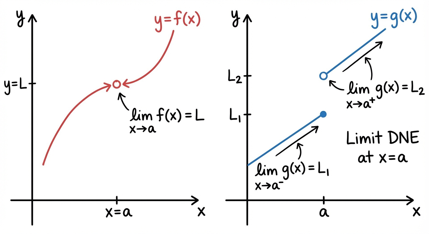
For a general limit to exist, the function must approach the same height from both the left and the right sides.

• Left-Hand Limit: Approaching $c$ from values smaller than $c$. Notation: $\lim_{x \to c^-} f(x)$
• Right-Hand Limit: Approaching $c$ from values larger than $c$. Notation: $\lim_{x \to c^+} f(x)$

The General Limit Existence Theorem:
$\lim{x \to c} f(x) = L$ if and only if: \lim{x \to c^-} f(x) = \lim_{x \to c^+} f(x) = L

If the left and right approaches do not match, the limit Does Not Exist (DNE).

Estimating Limits Graphically and Numerically

Graphical Estimation

When given a graph, trace the function with your finger approaching the x-value in question from both sides.

• Holes: If the graph has a holes at $x=c$, the limit is the y-value of the hole.
• Jumps: If the graph breaks, the limit DNE.
• Vertical Asymptotes: If the graph shoots up or down infinitely, the limit is $\infty$, $-\infty$, or DNE (depending on direction).

Numerical Estimation (Tables)

To estimate $\lim_{x \to 2} f(x)$, plug in x-values increasingly close to 2 from both sides:

In this table, it is clear that as x approaches 2, f(x) approaches 4.

Determining Limits Algebraically

1. Direct Substitution (The First Step)

Always try to plug the number $c$ into the function first.

• If you get a real number (e.g., $5$, $0$, $1/2$), that is your answer.
• If you get $\frac{k}{0}$ (where $k \neq 0$), a vertical asymptote exists (limit is $\pm\infty$ or DNE).
• If you get $\frac{0}{0}$, this is an Indeterminate Form. It means a hole likely exists, and you must use algebraic manipulation to find the true value.

2. Solving Indeterminate Forms ($0/0$)

When direct substitution yields $\frac{0}{0}$, use these techniques:

A. Factoring and Canceling
Useful for polynomials. Factor the numerator and denominator, cancel the common factor (the removable discontinuity), then retry substitution.

Example: Find $\lim{x \to 3} \frac{x^2 - 9}{x - 3}$ \lim{x \to 3} \frac{(x-3)(x+3)}{x-3} = \lim_{x \to 3} (x+3) = 3 + 3 = 6

B. Rationalization (Conjugates)
Useful for square roots. Multiply the numerator and denominator by the conjugate of the expression containing the root.

Example: $\lim_{x \to 0} \frac{\sqrt{x+4}-2}{x}$
Multiplied by conjugate $\frac{\sqrt{x+4}+2}{\sqrt{x+4}+2}$ simplifies to $\frac{1}{2+2} = \frac{1}{4}$.

C. Complex Fractions
If the function contains fractions within fractions, find a common denominator to combine them into a single numerator/denominator structure.

3. Special Trigonometric Limits

Memorize these two standard limits as $x \to 0$:

1. \lim_{x \to 0} \frac{\sin x}{x} = 1
2. \lim_{x \to 0} \frac{1 - \cos x}{x} = 0

Generalization for coefficients: $\lim_{x \to 0} \frac{\sin(ax)}{bx} = \frac{a}{b}$

The Squeeze Theorem (Sandwich Theorem)

If you cannot evaluate a limit directly, you may be able to "squeeze" it between two known functions.

Theorem Statement:
If $g(x) \leq f(x) \leq h(x)$ for all $x$ in an open interval containing $c$ (except possibly at $c$), and:
\lim{x \to c} g(x) = \lim{x \to c} h(x) = L
Then:
\lim_{x \to c} f(x) = L

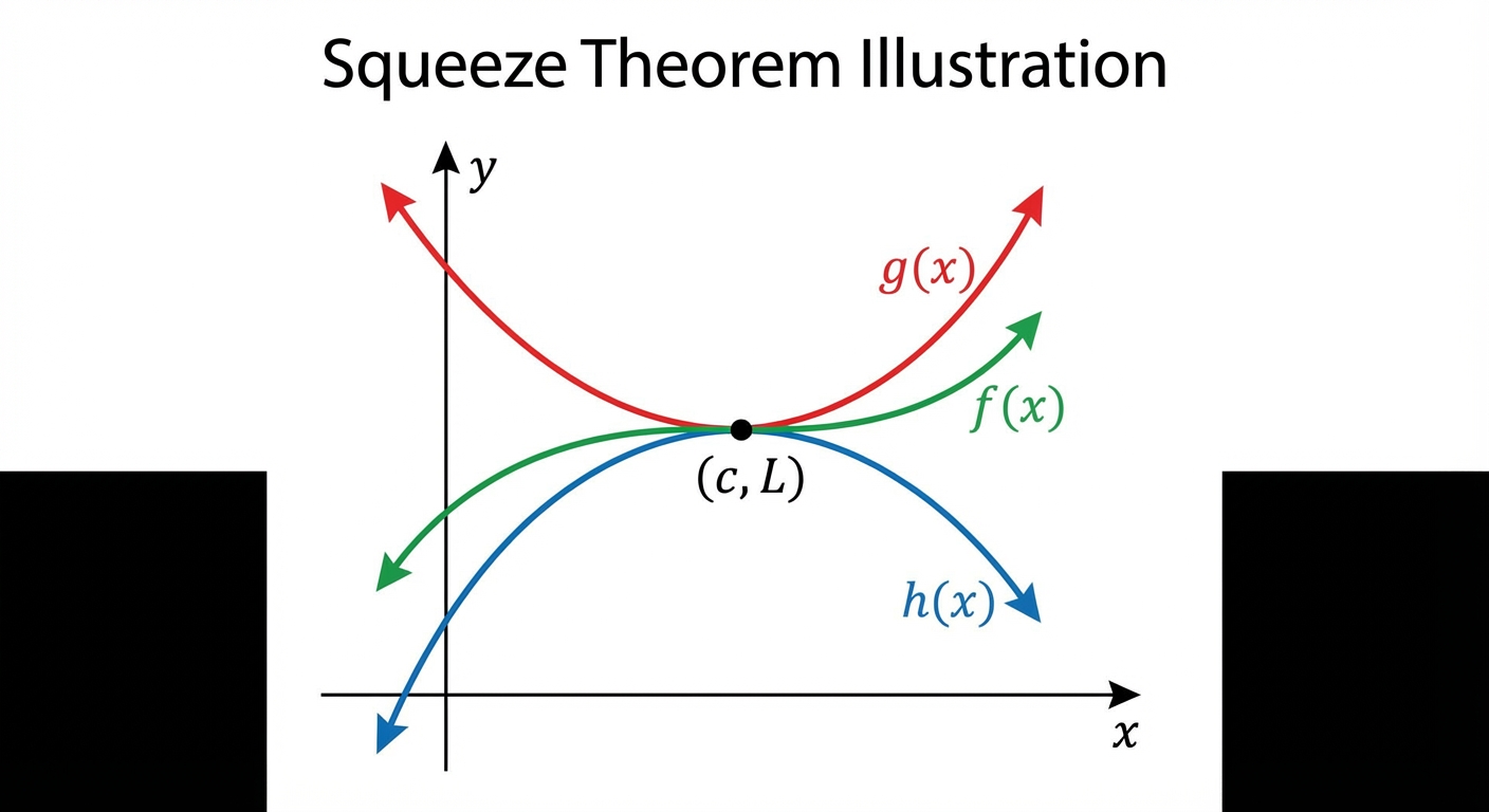
Common Application: Limits involving $\sin(\frac{1}{x})$ or $\cos(\frac{1}{x})$, which oscillate wildly.
Example: $\lim_{x \to 0} x^2 \sin(\frac{1}{x}) = 0$ because $-x^2 \le x^2 \sin(\frac{1}{x}) \le x^2$.

Continuity

Continuity is one of the most frequently tested concepts on the AP exam. A function includes no breaks, jumps, or holes.

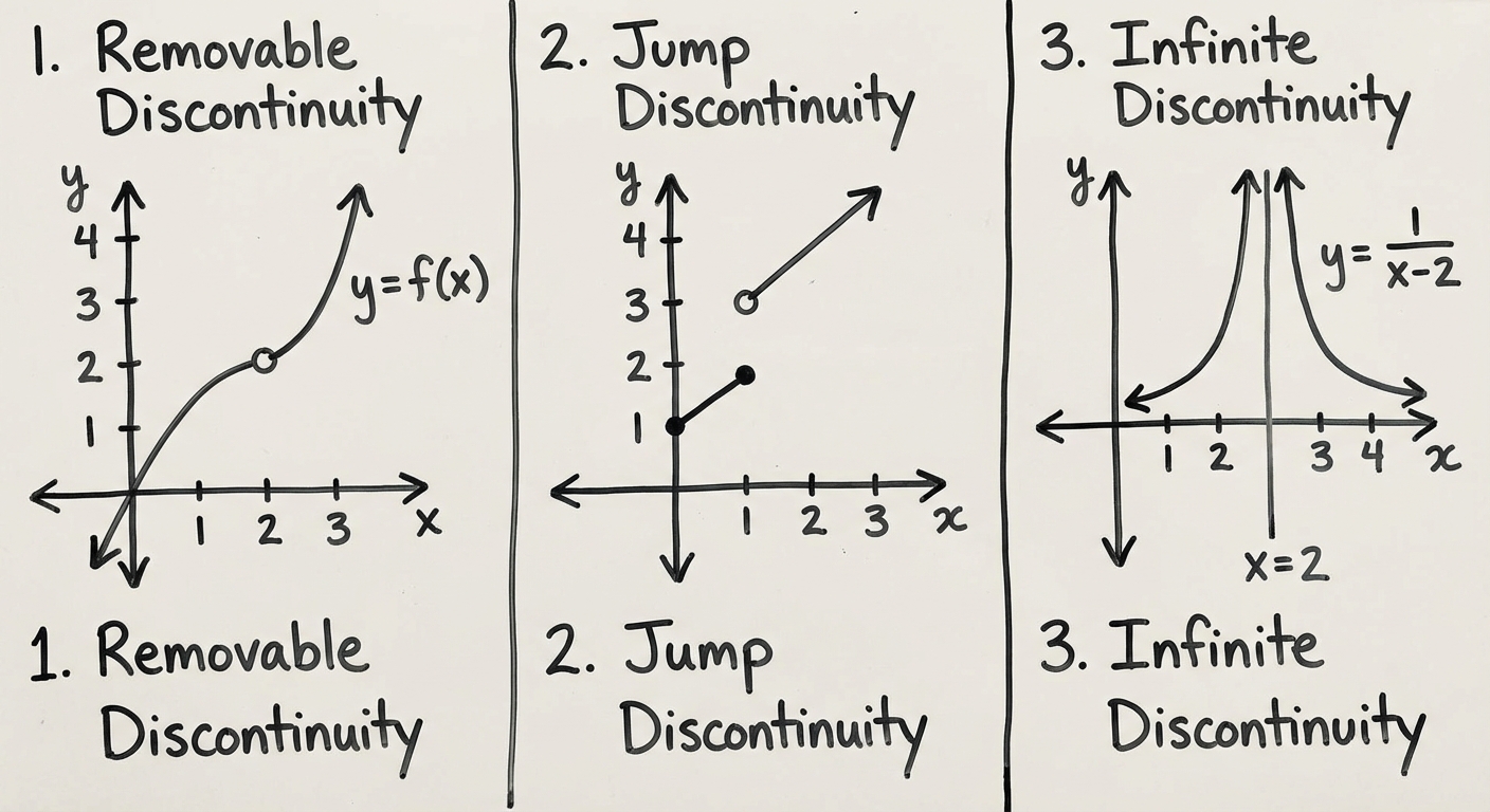
Types of Discontinuities

1. Removable Discontinuity (Hole): The limit exists, but $f(c)$ is either undefined or practically different from the limit. Algebraically, these occur when factors cancel.
2. Jump Discontinuity: $\lim{x \to c^-} f(x) \neq \lim{x \to c^+} f(x)$. Common in piecewise functions or step functions (e.g., $|x|/x$).
3. Infinite Discontinuity (Vertical Asymptote): One or both one-sided limits go to $\pm\infty$.

The Definition of Continuity (The 3-Step Test)

For a function $f(x)$ to be continuous at a point $x=c$, ALL three conditions must be met:

1. $f(c)$ is defined (The point exists).
2. $\lim_{x \to c} f(x)$ exists (Left limit = Right limit).
3. $\lim_{x \to c} f(x) = f(c)$ (The limit equals the function value).

If a question asks you to "Prove continuity," you must explicitly show all three steps.

Removing Discontinuities

Simplifying a rational function by canceling terms creates a new function that is continuous at the "hole." This is often called the Extended Function.

Asymptotes and Limits at Infinity

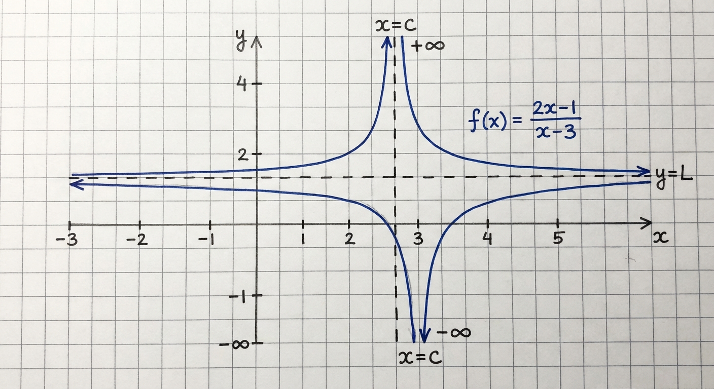
Vertical Asymptotes (Infinite Limits)

A line $x = c$ is a vertical asymptote if $\lim_{x \to c} f(x) = \pm\infty$.

• This occurs when the denominator is 0 but the numerator is not.
• Note: Infinite limits strictly rarely "exist" as a real number, but on the AP exam, we describe the behavior as $\infty$ or $-\infty$.

Horizontal Asymptotes (Limits at Infinity)

A line $y = L$ is a horizontal asymptote if:
\lim{x \to \infty} f(x) = L \quad \text{OR} \quad \lim{x \to -\infty} f(x) = L

These limits describe the End Behavior of the function.

Rules for Rational Functions: $\frac{P(x)}{Q(x)}$
Compare the degree (highest exponent) of the numerator ($N$) and denominator ($D$).

1. Bottom Heavy ($N < D$): Limit is 0. (Horizontal Asymptote: $y=0$)
   • Ex: $\lim_{x \to \infty} \frac{3x}{x^2+1} = 0$
2. Equations ($N = D$): Limit is the Ratio of Leading Coefficients.
   • Ex: $\lim_{x \to \infty} \frac{4x^3 - 1}{2x^3 + 5} = \frac{4}{2} = 2$. (HA: $y=2$)
3. Top Heavy ($N > D$): Limit is $\pm\infty$ (DNE). There is no horizontal asymptote (often a slant asymptote).

Note on Exponentials:
Remember that $e^x$ grows faster than any polynomial.

• $\lim_{x \to \infty} \frac{x^{100}}{e^x} = 0$

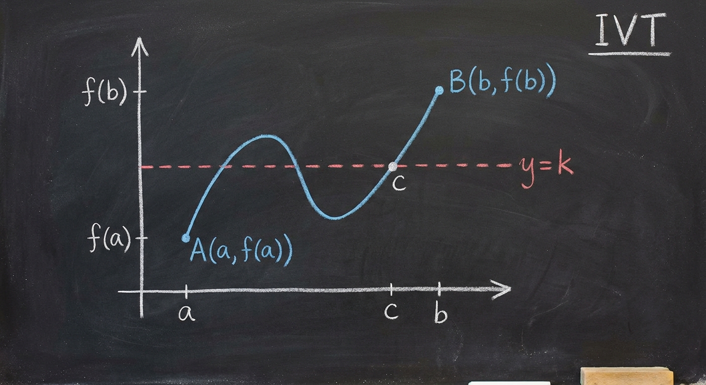
Intermediate Value Theorem (IVT)

The IVT is an "Existence Theorem." It doesn't tell you what the value is or where it is, only that it exists.

Conditions:

1. $f(x)$ is continuous on the closed interval $[a, b]$.

Conclusion:
If $k$ is any number between $f(a)$ and $f(b)$, then there exists at least one number $c$ in $(a, b)$ such that $f(c) = k$.

Real World Analogy: If you were 3 feet tall at age 5, and 5 feet tall at age 12, there must have been a moment when you were exactly 4 feet tall (assuming growth is continuous).

Typical Exam Problem: "Show that $f(x) = x^3 + x - 1$ has a zero on the interval $[0, 1]$."

1. Check continuity (Polynomials are continuous everywhere).
2. Find $f(0) = -1$.
3. Find $f(1) = 1$.
4. Since $-1 < 0 < 1$, by IVT, there is a $c$ where $f(c) = 0$.

Common Mistakes & Pitfalls

1. The "0/0" Answer: Never write "0/0" as a final answer. It is an instruction to do more work (factor, conjugate, etc.).
2. Confusing Limit Value vs. Function Value: A limit is about the journey (approach); the function value is the destination. A limit can exist even if the function is undefined at that point (a hole).
3. Mismatched Indices in One-Sided Limits: Notation matters. $\lim{x \to 2^-}$ is NOT the same as $\lim{x \to -2}$. The minus sign in superscript means "from the left."
4. Forgetting Conditions for IVT: You cannot apply the Intermediate Value Theorem unless you state that the function is continuous on the interval.
5. Substituting Infinity: Infinity is not a number. Do not write arithmetic like $\frac{1}{\infty}$. Instead, reason that "1 divided by a huge number approaches 0."