Mastering Kinematics: The Science of One-Dimensional Motion
Scalars and Vectors in Linear Systems
To understand how objects move, we must first learn the language of physics. In AP Physics 1, quantities are categorized into two fundamental types based on whether direction matters. This distinction is critical because Kinematics (the description of motion) relies heavily on vector analysis, even in just one dimension.
Defining the Terms
- Scalars: Quantities that are fully described by a magnitude (numerical value) only. Examples include time, mass, speed, and distance.
- Vectors: Quantities that are fully described by both a magnitude and a direction. Examples include displacement, velocity, acceleration, and force.
Direction in One Dimension
In 1D motion (motion along a straight line), direction is represented algebraically using positive ($+$) and negative ($-$) signs.
- Positive ($+$) usually implies: Right, Up, East, or Forward.
- Negative ($-$) usually implies: Left, Down, West, or Backward.
Note: The choice of which direction is positive is arbitrary (you can define Down as positive if you want), but once chosen, you must remain consistent throughout the problem.
Displacement, Velocity, and Acceleration
Movement is broken down into three layers of abstraction: where you are, how fast you are changing position, and how fast you are changing your speed.
Position, Distance, and Displacement
- Position ($x$): The specific location of an object relative to a defined origin ($x=0$).
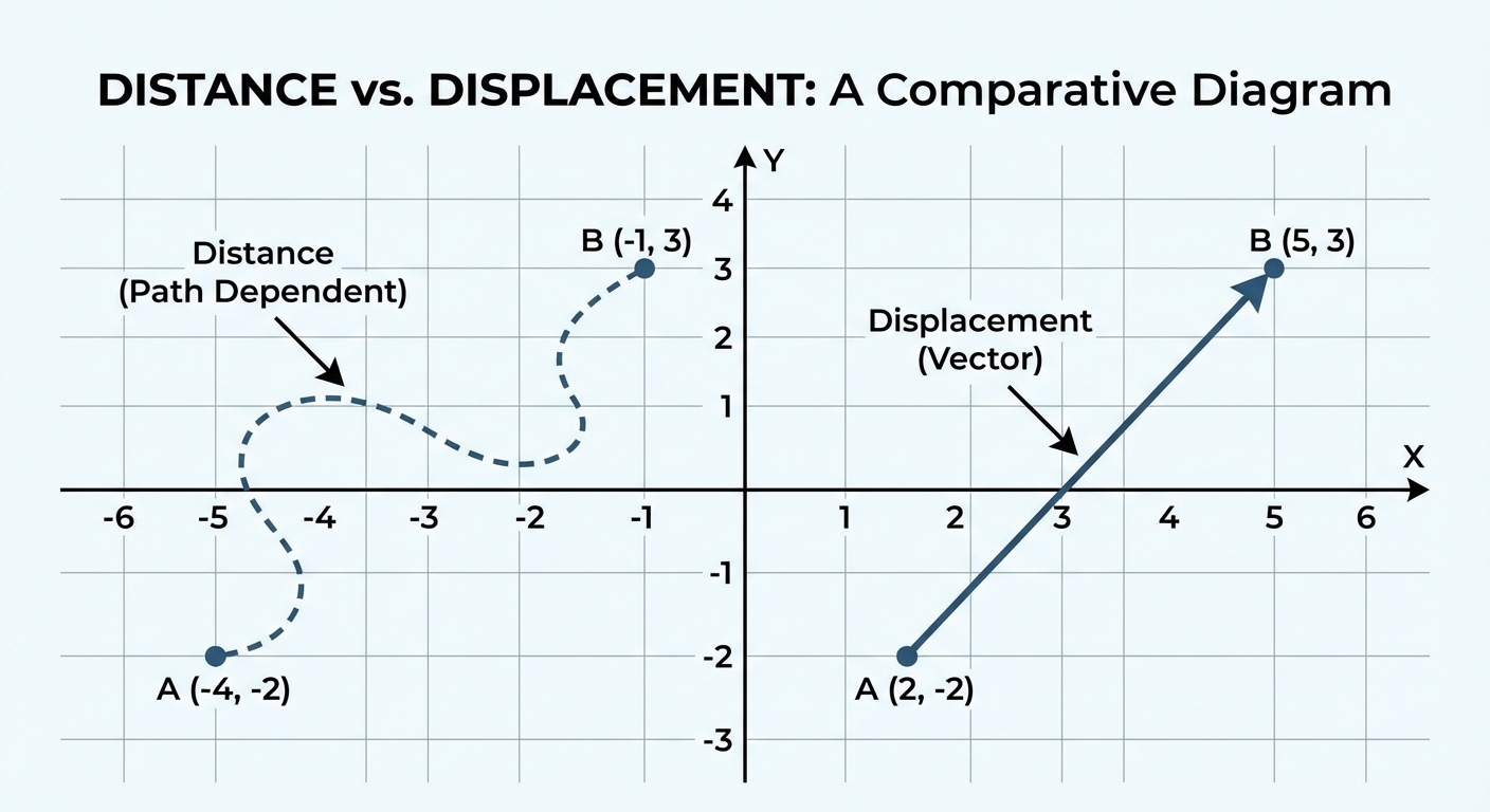
- Distance ($d$): A scalar representing the total length of the path traveled. It is path-dependent and always positive.
- Displacement ($\Delta x$): A vector representing the straight-line change in position. It is path-independent.
Where $xf$ is the final position and $xi$ is the initial position.
Speed vs. Velocity
Just as distance differs from displacement, speed differs from velocity.
- Average Speed: The total distance traveled divided by the total time elapsed. (Scalar)
- Average Velocity ($\bar{v}$): The displacement divided by the time interval. (Vector)
\bar{v} = \frac{\Delta x}{\Delta t} =
\frac{xf - xi}{tf - ti}
Acceleration ($a$)
Acceleration is the rate of change of velocity. It is a vector, meaning it has both magnitude and direction.
The Signs of Velocity and Acceleration
A common point of confusion is how velocity and acceleration interact. The sign of acceleration alone does not tell you if an object is speeding up or slowing down; you must compare it to the sign of velocity.
| Velocity ($v$) | Acceleration ($a$) | Resulting Motion |
|---|---|---|
| Positive ($+$) | Positive ($+$) | Speeding Up (in positive direction) |
| Negative ($-$) | Negative ($-$) | Speeding Up (in negative direction) |
| Positive ($+$) | Negative ($-$) | Slowing Down |
| Negative ($-$) | Positive ($+$) | Slowing Down |
Mnemonic: If the signs Agree, the object Accelerates (speeds up). If the signs are Opposite, the object is Opposed (slows down).
Representing Motion
AP Physics 1 requires you to translate between multiple representations of motion: verbal descriptions, mathematical equations, motion diagrams, and graphs.
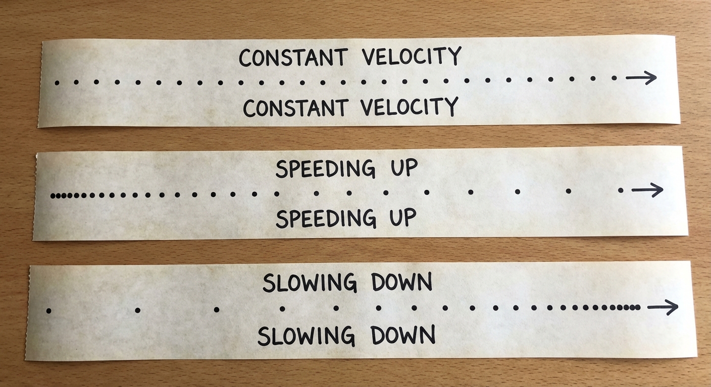
1. Motion Diagrams (Dot Diagrams)
These diagrams visualize the position of an object at equal time intervals (like a strobe light photo).
- Constant Velocity: Dots are spaced equally apart.
- Speeding Up: Spacing between dots increases.
- Slowing Down: Spacing between dots decreases.
2. Kinematic Graphs
Understanding slope and area is the key to mastering graphical analysis.
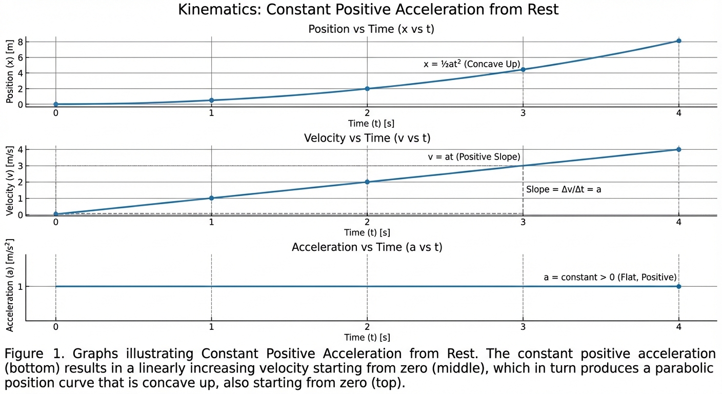
Position-Time Graphs ($x$ vs. $t$)
- Slope: Represents Velocity.
- Straight line = Constant velocity.
- Curved line = Changing velocity (acceleration).
- Concavity: Indicates the sign of acceleration.
- Concave Up (looks like a cup $\cup$): Positive Acceleration.
- Concave Down (looks like a frown $\cap$): Negative Acceleration.
Velocity-Time Graphs ($v$ vs. $t$)
This is the most information-dense graph.
- Slope: Represents Acceleration.
- Area Under the Curve: Represents Displacement ($\Delta x$).
- Area above the $t$-axis is positive displacement.
- Area below the $t$-axis is negative displacement.
Exam Tip: If a $v$ vs. $t$ graph crosses the horizontal axis ($v=0$), the object has changed direction.
Acceleration-Time Graphs ($a$ vs. $t$)
- Area Under the Curve: Represents Change in Velocity ($\Delta v$).
- In AP Physics 1, we mostly deal with constant acceleration, so these graphs are usually horizontal lines.
3. The Kinematic Equations (UAM)
When acceleration is constant (Uniform Accelerated Motion or UAM), we can use the following derived equations. These are provided on your AP Table of Information.
Velocity as a function of time:
Position as a function of time:
Velocity related to position (Time-independent):
Variables Key:
- $v_x$ = final velocity
- $v_{x0}$ = initial velocity
- $a_x$ = acceleration
- $t$ = time interval
- $x - x_0$ = displacement
4. Worked Example: The Braking Car
Problem: A car traveling at $20 \text{ m/s}$ spots a hazard and hits the brakes, accelerating at $-5 \text{ m/s}^2$. How far does it travel before stopping?
Solution:
- Identify Knowns: $v{x0} = 20 \text{ m/s}$, $vx = 0 \text{ m/s}$ (stopped), $a_x = -5 \text{ m/s}^2$.
- Identify Unknown: Displacement ($x - x_0$).
- Select Equation: We don't have time ($t$), so we use the time-independent equation:
- Substitute and Solve:
Common Mistakes & Pitfalls
- The "Negative Acceleration" Trap: Students often assume negative acceleration always means "slowing down." Remember: if velocity is negative and acceleration is negative, the object is speeding up in the negative direction.
- Mixing Distance and Displacement: In equations like , you must use displacement. If you run a $400\text{m}$ circular track and finish where you started, your average velocity is $0$, even though your speed was non-zero.
- Top of the Motion: When an object is thrown straight up, at the very peak of its flight, its velocity is zero, but its acceleration is NOT zero. Gravity is still pulling down at $9.8 \text{ m/s}^2$. If acceleration were zero, the object would hover perpendicular in the air forever.
- Graph Confusion: Don't just look at the shape of the line; check the axes first. A flat horizontal line means "stopped" on a Position-Time graph, but it means "constant velocity" on a Velocity-Time graph.