AP Computer Science Principles: Big Idea 2 — Data and Information
Topic 2.1: Binary Numbers and Data Representation
In the world of computer science, everything starts at the lowest level of abstraction: the bit. Understanding how complex information—like the video you watch or the text you are reading right now—is reduced to simple electrical signals is fundamental to this course.
Binary Numbers & Digital Data
The Atom of Computing: The Bit
A Bit (short for Binary digit) is the smallest unit of data in a computer. It can hold one of two values: 0 or 1.
Computers use bits because they operate on electricity, which can be easily measured in two states: On (1) or Off (0).
- Byte: A group of 8 bits.
- Abstraction: Bits are grouped together to represent larger, more complex data like numbers, characters, and colors. This grouping is an abstraction that hides the complexity of the hardware from the user.
Number Systems: Decimal vs. Binary
Humans use the Decimal System (Base 10), likely because we have ten fingers. We use digits 0–9. Computers use the Binary System (Base 2), using only 0 and 1.
To understand binary, helpful to recall how place value works:
Decimal (Base 10):
Binary (Base 2):
Binary uses positions based on powers of 2.
| Power of 2 | $2^7$ | $2^6$ | $2^5$ | $2^4$ | $2^3$ | $2^2$ | $2^1$ | $2^0$ |
|---|---|---|---|---|---|---|---|---|
| Decimal Value | 128 | 64 | 32 | 16 | 8 | 4 | 2 | 1 |
Analog vs. Digital Data
Not all data in the real world is binary. The physical world is Analog.
- Analog Data: Continuous, infinite stream of values that change smoothly over time (e.g., sound waves, temperature, colors in a painting).
- Digital Data: Discrete, finite values (e.g., an MP3 file, a JPEG image).
To store analog data on a computer, we must perform Sampling. This involves measuring the analog signal at regular intervals and recording the value as a number.
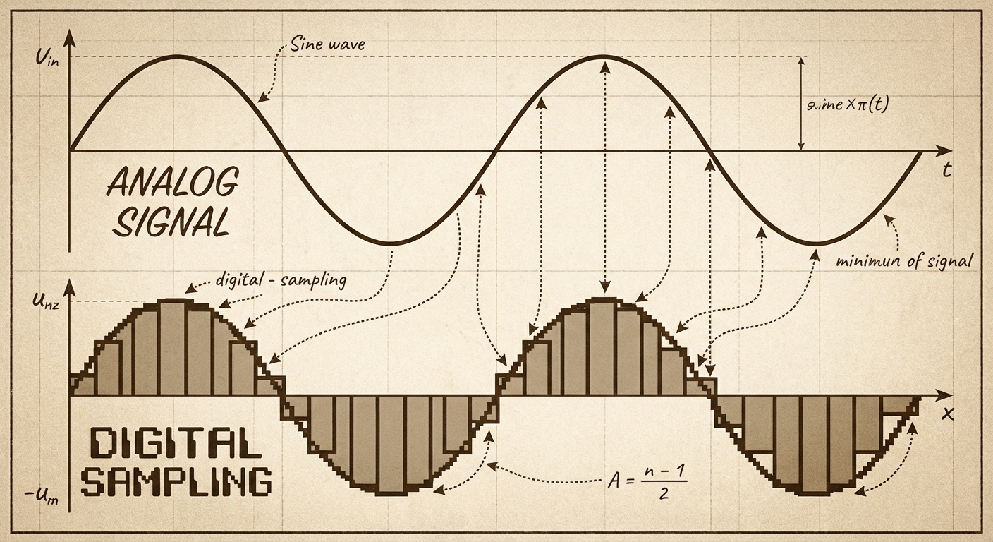
- Sampling Rate: How often you measure the data. Higher sampling rates = better quality but larger file sizes.
- Bit Depth: How many bits represent each sample. More bits = more precision but larger file sizes.
Limitations of Finite Representation
Because computer memory is fixed (e.g., 32-bit or 64-bit integers), we cannot represent every number perfectly.
Overflow Error: This occurs when a calculation produces a result larger than the space allocated to store it.
- Analogy: Imagine a car odometer that only goes up to 999,999. If you drive one more mile, it resets to 000,000. That reset is an overflow.
- Code Limit: If you have 4 bits, the max value is 15 ($11112$). If you add 1, you get 16 ($100002$), but the computer drops the 5th bit, resulting in 0.
Round-off Error: Occurs attempting to represent precise decimal values (floating-point numbers). Because binary cannot perfectly represent certain fractions (like 0.1 or $\frac{1}{3}$), the number is rounded to the nearest representable value.
- Impact: While usually small, these errors can accumulate in simulations or financial calculations, leading to significant inaccuracies.
Topic 2.2: Data Compression
As we digitize the world, file sizes grow massive. Data Compression is the process of encoding information using fewer bits than the original representation. This saves storage space and reduces transmission time across the internet.
There are two fundamental approaches: Lossless and Lossy.
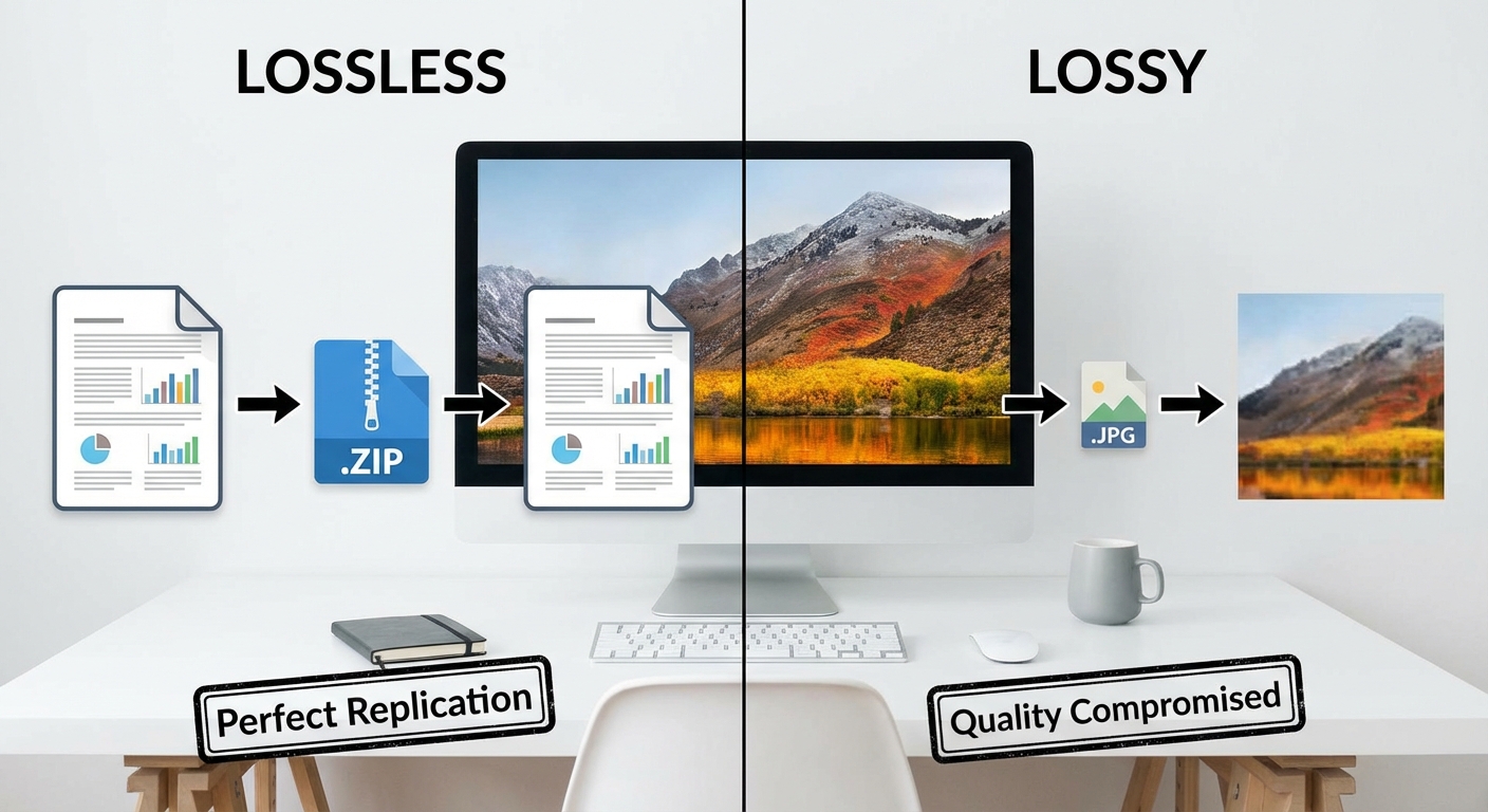
1. Lossless Compression
Lossless compression algorithms reduce the number of bits needed without losing any information. The original file can be perfectly reconstructed.
- Mechanism: It looks for redundancy (patterns) and creates a dictionary or key to represent them.
- Example:
- Original:
BBAAAAAAACCCCCC - Compressed (Run-Length Encoding):
2B7A6C
- Original:
- Use Cases: Text files, executable software code, bank records. (You wouldn't want a bank transfer to "approximately" match the original amount!)
- Limitation: Often cannot achieve as high a compression (reduction) ratio as lossy methods.
2. Lossy Compression
Lossy compression significantly reduces the number of bits by throwing away some information. The original file cannot be perfectly reconstructed.
- Mechanism: It discards data that human perception is less likely to notice (e.g., heavy compression might remove sounds outside the range of human hearing or subtle color variations).
- Use Cases: Images (JPEG), Audio (MP3), Video (MP4).
- Trade-off: You sacrifice quality for a massive reduction in file size.
| Feature | Lossless | Lossy |
|---|---|---|
| Restorability | Perfect replica of original | Approximation of original |
| File Size Reduction | Low to Medium | High |
| Best For | Text, Code, Important Data | Multimedia (Images, Sound, Video) |
Topic 2.3: Extracting Information from Data
Having data represented in bits is useless unless we can turn it into insight. The progression is: Data $\rightarrow$ Information $\rightarrow$ Knowledge.
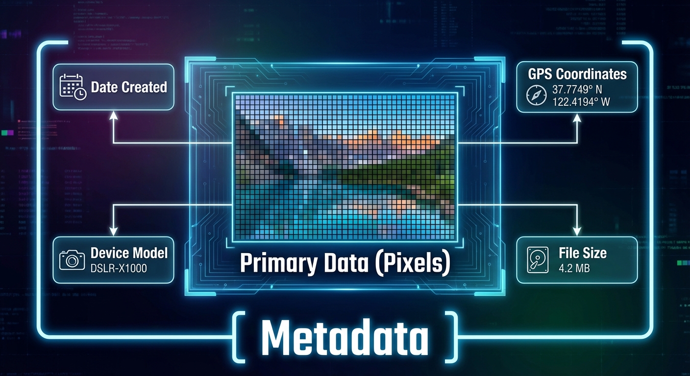
Metadata: Data about Data
Metadata is descriptive data about an image, a web page, or other complex objects.
- Examples: The date a photo was taken, valid shutter speed, GPS location, author name, file size.
- Key Concept: Changing the metadata does not change the visual content of the image, but it can make the data harder to find or verify.
- Security: Metadata can leak privacy (e.g., posting a photo from home that includes GPS coordinates in the metadata).
Processing Data
To extract information, we often use tools to process large datasets. Key steps include:
- Cleaning Data: Removing corrupt data, fixing inconsistent formatting (e.g., "NY" vs "N.Y."), and handling missing values. Without cleaning, analysis is flawed.
- Filtering: Keeping only the rows that match certain criteria.
- Visualization: Using charts and graphs to identify trends that raw text tables hide.
The Golden Rule of Analysis: Correlation vs. Causation
This is a frequent exam pitfall.
- Correlation: A relationship where two variables move together (e.g., ice cream sales and shark attacks both go up in July).
- Causation: One variable causes the other to change.
Just because two data sets are correlated does NOT mean one caused the other. (In the example above, the cause for both is summer heat, not the ice cream causing shark attacks).
Bias in Data
Data processing is objective, but the data itself or the choice of data can be biased.
- If you only survey landline owners about technology use, you miss the mobile-only demographic.
- Algorithms trained on biased historical data will repeat those biases.
Summary of Common Mistakes
- Confusing Lossy and Lossless: Remember, use Lossless if you need the exact original back (like code). Use Lossy if you need to save massive space and "good enough" is okay (like a cat video).
- Assuming Digital is Perfect: Students often forget that converting analog to digital always results in some loss of detail due to sampling limits. It is never a perfect curve.
- Correlation = Causation: Never claim X causes Y just because the graphs look similar. Always check for other variables.
- Byte Math: Remember $2^{10}$ is 1024, not 1000. In CSP, approximations are often used, but know the specific powers of 2 for small numbers.
- Overflow: Thinking overflow just means "error". Specifically, it means the number is too big regarding the bit width.
Mnemonic for Metric Prefixes (Powers of 10 vs 2)
- Kilo: $1000$ (or $2^{10} \approx 1024$)
- Mega: $1,000,000$ (or $2^{20}$)
- Giga: $1,000,000,000$ (or $2^{30}$)
- Tera: $1,000,000,000,000$ (or $2^{40}$)