Differentiation: Definition and Fundamental Properties

Derivatives as Slopes and Rates of Change

What a derivative measures (two equivalent interpretations)

A derivative measures how a function changes right now, at a particular input. In algebra, you usually compute change over an interval using two points and the slope of a secant line. Calculus refines that idea by asking for the slope of the curve at a single point, which is defined as a limit of secant slopes as the second point moves in.

There are two perspectives you must be comfortable switching between:

1) Geometric (slope): the derivative at an input is the slope of the tangent line to the graph at that point.

2) Real-world (rate): the derivative at an input is the instantaneous rate of change of the output with respect to the input.

If the input represents time and the output represents position, then secant slopes are average velocities and the tangent slope is instantaneous velocity.

Average rate of change (difference quotient over an interval)

The average rate of change of a function from one input to another is the slope of the secant line through the two points.

If the interval is from input a to input b, the average rate of change is

\frac{f(b)-f(a)}{b-a}

You’ll also see this described informally as “change in output over change in input,” like

\frac{y_2-y_1}{x_2-x_1}

This is a rate of change over an interval of time (or distance, or whatever the input represents).

Instantaneous rate of change (difference quotient with a limit)

To get the instantaneous rate of change at a specific input, you shrink the interval until it becomes “infinitesimally small.” A standard way is to write the second input as a+h and take a limit as h approaches 0.

The secant slope becomes

\frac{f(a+h)-f(a)}{h}

and the instantaneous rate of change is the limit of that expression as h approaches 0.

Secant lines approximate, tangent lines model

For a straight (linear) graph, slope is constant and you can use “rise over run” anywhere. For a curved graph, the slope changes from point to point, so you approximate slope at a point by using a secant line through two nearby points. The closer the two points are, the more accurate the approximation.

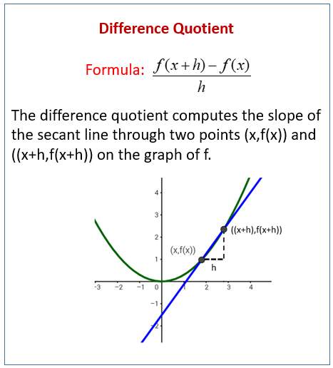
The true “slope at a point” is the slope of the tangent line, which you obtain by taking the limit of secant slopes (instantaneous rate of change).

Units and meaning of sign

If the function has units, the derivative has units of output per input. For example, if input is hours and output is miles, then the derivative has units miles per hour.

Also, the sign matters:

• Positive derivative means the function is increasing at that input.
• Negative derivative means the function is decreasing at that input.

Worked example: interpreting slope as a rate

Suppose T(t) is the temperature (degrees Celsius) of tea t minutes after pouring.

• The average cooling rate from 10 to 12 minutes is

\frac{T(12)-T(10)}{12-10}

• The instantaneous cooling rate at 10 minutes is T'(10).

If

T'(10)=-0.8

then at exactly 10 minutes, the tea is cooling at 0.8 degrees Celsius per minute.

Exam Focus

• Typical question patterns:
  • “Find the slope of the tangent line to y=f(x) at x=a using the definition of the derivative.”
  • “Interpret f'(a) in context (include units and meaning of sign).”
  • “Compute average rate of change on an interval and compare to instantaneous rate at an endpoint.”
• Common mistakes:
  • Confusing average rate of change with instantaneous rate (using a secant slope when asked for a derivative).
  • Forgetting units or misinterpreting a negative derivative (negative means decreasing, not “bad”).
  • Treating the tangent line as “touches once” rather than “has matching slope at the point.”

The Limit Definition of the Derivative (Difference Quotient)

Building the definition

To define the slope at a point, start with the slope between two points on the curve.

Take points

\left(a,f(a)\right)

and

\left(a+h,f(a+h)\right)

The slope of the secant line is

\frac{f(a+h)-f(a)}{(a+h)-a}

which simplifies to

\frac{f(a+h)-f(a)}{h}

As h approaches 0, the second point approaches the first. If the limit exists, that limiting slope is the derivative.

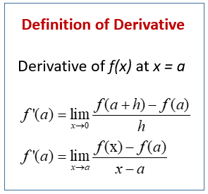
Formal definition (two equivalent forms)

The derivative of f at input a is

f'(a)=\lim_{h\to 0}\frac{f(a+h)-f(a)}{h}

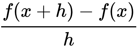
The expression is called a difference quotient.

An equivalent bookkeeping form is

f'(a)=\lim_{x\to a}\frac{f(x)-f(a)}{x-a}

One-sided derivatives

Sometimes behavior differs depending on direction. Define:

Right-hand derivative:

f'_+(a)=\lim_{h\to 0^+}\frac{f(a+h)-f(a)}{h}

Left-hand derivative:

f'_-(a)=\lim_{h\to 0^-}\frac{f(a+h)-f(a)}{h}

For the (two-sided) derivative f'(a) to exist, both one-sided derivatives must exist and be equal.

Why you cannot plug in immediately

The difference quotient is undefined at h=0, so you cannot substitute h=0 right away. The goal is to simplify the expression so that a factor causing the undefined form cancels, and then take the limit.

This is why derivative-from-definition problems often require factoring, expanding, simplifying, or rationalizing.

Worked example 1: derivative of a quadratic

Let

f(x)=x^2

Find f'(a) from the definition.

Start:

f'(a)=\lim_{h\to 0}\frac{f(a+h)-f(a)}{h}

Compute:

f(a+h)=(a+h)^2=a^2+2ah+h^2

f(a)=a^2

Substitute:

f'(a)=\lim_{h\to 0}\frac{(a^2+2ah+h^2)-a^2}{h}

Simplify:

f'(a)=\lim_{h\to 0}\frac{2ah+h^2}{h}

Factor and cancel (valid for h\neq 0 in the limit process):

f'(a)=\lim_{h\to 0}(2a+h)

Take the limit:

f'(a)=2a

So the derivative function is

f'(x)=2x

Worked example 2: rationalizing a radical

Let

f(x)=\sqrt{x}

Find f'(a) from the definition.

f'(a)=\lim_{h\to 0}\frac{\sqrt{a+h}-\sqrt{a}}{h}

Multiply by the conjugate:

f'(a)=\lim_{h\to 0}\frac{\sqrt{a+h}-\sqrt{a}}{h}\cdot\frac{\sqrt{a+h}+\sqrt{a}}{\sqrt{a+h}+\sqrt{a}}

Use difference of squares:

f'(a)=\lim_{h\to 0}\frac{(a+h)-a}{h(\sqrt{a+h}+\sqrt{a})}

Simplify and cancel:

f'(a)=\lim_{h\to 0}\frac{1}{\sqrt{a+h}+\sqrt{a}}

Now substitute h=0:

f'(a)=\frac{1}{2\sqrt{a}}

Exam Focus

• Typical question patterns:
  • “Use the definition to find f'(a) for a given function (often polynomial or radical).”
  • “Write the difference quotient for f and simplify.”
  • “Compute f'(a) at a specific number using the limit definition.”
• Common mistakes:
  • Plugging in h=0 too early (before simplifying to remove the removable discontinuity).
  • Algebra errors when expanding f(a+h) (especially binomial squares/cubes).
  • Canceling terms incorrectly (you can cancel a factor of h, not an h that’s part of a sum).

Derivative Notation and the Derivative as a Function

Notation you must recognize and translate

You will see multiple notations for derivatives. They all refer to the same concept, but different contexts prefer different symbols.

Derivative at a specific input (a single number):

f'(a)

y'(a)

\left.\frac{dy}{dx}\right|_{x=a}

Derivative function (a new function giving slopes/rates for all inputs):

f'(x)

y'

\frac{dy}{dx}

Second derivative (derivative of the derivative):

f''(x)

\frac{d^2y}{dx^2}

You may also see the same pattern with different function names, such as g(x) having derivative g'(x) and second derivative g''(x).

The derivative as a new function

Computing f'(a) produces one slope at one point. Computing f'(x) produces a whole function that tells you the slope (or instantaneous rate) at every input where the derivative exists.

Thinking of the derivative as a function lets you evaluate, graph, and analyze it to understand where the original function increases, decreases, or has horizontal tangents.

Connecting graphs of a function and its derivative

These qualitative relationships are essential:

• If the function is increasing at an input, the derivative is positive there.
• If the function is decreasing at an input, the derivative is negative there.
• If the function has a horizontal tangent, the derivative equals 0 there.

Important subtlety: a derivative equal to 0 guarantees a horizontal tangent, but it does not automatically guarantee a maximum or minimum.

Estimating derivatives from tables (secant slopes near the point)

Given a table, you approximate the derivative using nearby points. A common, often more accurate method is the symmetric difference quotient. If you have values at inputs a-h and a+h, then

f'(a)\approx\frac{f(a+h)-f(a-h)}{2h}

If the table isn’t symmetric or spacing isn’t uniform, use the closest points you have and clearly state which secant slope you used.

Worked example 1: estimating from a table

Given

f(1.9)=5.74

f(2.0)=5.99

f(2.1)=6.25

Estimate f'(2.0) using a symmetric difference with h=0.1:

f'(2.0)\approx\frac{f(2.1)-f(1.9)}{0.2}

f'(2.0)\approx\frac{6.25-5.74}{0.2}

f'(2.0)\approx 2.55

Estimating derivatives from graphs (tangent slope)

On a graph, the derivative value at an input is the slope of the tangent line. Practically, you sketch the tangent line at the point and compute rise over run using two readable points on that tangent line.

A frequent error is using two points on the curve near the point, which gives a secant slope instead.

Tangent line from function value and derivative value

If you know the point and the slope at that point, use point-slope form.

Worked example 2: tangent line equation

If

f(3)=10

and

f'(3)=-2

then the tangent line at input 3 is

y-10=-2(x-3)

which simplifies to

y=-2x+16

Exam Focus

• Typical question patterns:
  • “Given a table or graph of f, estimate f'(a).”
  • “Given f(a) and f'(a), find the equation of the tangent line.”
  • “Interpret f'(a) (sign, magnitude, and units) in a contextual problem.”
• Common mistakes:
  • Mixing up f(a) and f'(a) (using slope where a function value is needed, or vice versa).
  • Estimating slope from points on the curve instead of points on the tangent line.
  • Forgetting that an approximation should be labeled as approximate (especially from tables/graphs).

Differentiability and Continuity

What it means to be differentiable

A function is differentiable at an input if its derivative exists there as a finite real number. Intuitively, differentiability means the graph is not only unbroken at that point, but also smooth enough to have a well-defined (non-vertical) tangent slope.

Differentiability implies continuity (but not conversely)

A key theorem:

• If a function is differentiable at an input, then it is continuous at that input.

A very useful contrapositive:

• If a function is not continuous at an input, then it is not differentiable there.

But the converse is false:

• A function can be continuous yet not differentiable.

Common ways derivatives fail to exist

Derivatives often fail at:
1) Discontinuities (jump, infinite, removable)
2) Corners (left and right slopes approach different finite values)
3) Cusps (slopes become unbounded with opposite signs)
4) Vertical tangents (slopes become unbounded with the same sign)

The unifying idea is that the one-sided derivatives do not match, or the limiting slope is not finite.

One-sided derivatives and a classic corner

For the absolute value function at 0, the graph is continuous but has a corner.

Consider

f(x)=|x|

At input 0, the right-hand slope is 1 and the left-hand slope is negative 1, so the derivative does not exist there.

Worked example: differentiability at a piecewise point

Define the function as follows:

For inputs less than 1:

f(x)=x+2

For inputs greater than or equal to 1:

f(x)=3x

To be differentiable at input 1, the function must first be continuous.

Left-hand value at 1:

\lim_{x\to 1^-}f(x)=1+2=3

Right-hand value and actual value at 1:

f(1)=3\cdot 1=3

So it is continuous at 1.

Now compare one-sided derivatives:

• For inputs less than 1, the slope is 1.
• For inputs greater than 1, the slope is 3.

Because these do not match, the derivative at 1 does not exist. The graph is continuous there but has a corner.

Quick graph checklist for differentiability

When deciding from a graph whether a function is differentiable at a point:

• Is there a break or hole? If yes, not differentiable.
• Is there a sharp point (corner or cusp)? If yes, not differentiable.
• Is the tangent vertical? Then the derivative is not a finite real number.

Exam Focus

• Typical question patterns:
  • “At what inputs is f not differentiable? Justify using a graph.”
  • “Given a piecewise function, find values of constants so that f is continuous and differentiable at a point.”
  • “Explain why differentiability implies continuity (or apply the contrapositive).”
• Common mistakes:
  • Assuming “continuous” automatically means “differentiable.”
  • Missing corners on graphs because the curve looks smooth when not zoomed in.
  • Saying a vertical tangent means derivative equals 0 (the slope is unbounded, not flat).

Fundamental Derivative Rules (Linearity and the Power Rule)

Why we use rules

The limit definition gives the meaning of the derivative, but using it for every function is slow. Derivative rules are shortcuts proven from the definition, and they let you differentiate efficiently.

In this unit, the key rule set includes:

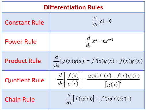
• Constant rule
• Constant multiple rule
• Power rule
• Sum and difference rules

These are often grouped as linearity properties.

Constant rule

If a function is constant, its slope is 0 everywhere:

\frac{d}{dx}(c)=0

Example: if

f(x)=10

then

f'(x)=0

Constant multiple rule

A constant factor pulls out of the derivative:

\frac{d}{dx}(cf(x))=c\cdot f'(x)

Sum and difference rules

Derivatives distribute over addition and subtraction:

\frac{d}{dx}(f(x)+g(x))=f'(x)+g'(x)

\frac{d}{dx}(f(x)-g(x))=f'(x)-g'(x)

Power rule

For powers of the input variable, the basic rule is

\frac{d}{dx}(x^n)=nx^{n-1}

A helpful description is: multiply down and decrease the power.

Examples:

\frac{d}{dx}(x^4)=4x^3

\frac{d}{dx}(2x^2)=4x

The power rule works for polynomials and also for negative integer exponents.

Worked example 1: differentiating a polynomial

Let

f(x)=5x^4-3x^2+7x-9

Differentiate term-by-term:

f'(x)=20x^3-6x+7

Worked example 2: negative exponents

Let

g(x)=2x^{-3}-x^{-1}

Then

g'(x)=-6x^{-4}+x^{-2}

Equivalently, with positive exponents:

g'(x)=-\frac{6}{x^4}+\frac{1}{x^2}

Common pitfalls with early rules

A frequent mistake is forgetting to subtract 1 from the exponent:

\frac{d}{dx}(x^n)\neq nx^n

Another common trap is trying to use the power rule on an unexpanded sum inside parentheses, such as differentiating

(x+1)^2

as if it were a simple power of the variable. That requires the chain rule (a later topic). In this unit, expand first:

(x+1)^2=x^2+2x+1

then differentiate.

Exam Focus

• Typical question patterns:
  • “Find f'(x) for a polynomial or a function with negative powers.”
  • “Find f'(a) by first finding f'(x) then evaluating.”
  • “Write the derivative and interpret it as a rate of change.”
• Common mistakes:
  • Using the power rule on expressions that are not simple powers of the variable (like (2x-1)^5 ) without expanding (this is really a chain rule situation).
  • Dropping signs when differentiating terms like -3x^2.
  • Forgetting constants differentiate to 0 and incorrectly carrying them through.

The Product Rule and Quotient Rule

Why these rules are needed

Linearity rules do not apply to multiplication or division. In particular, it is not true that the derivative of a product equals the product of derivatives.

Wrong idea:

\frac{d}{dx}(f(x)g(x))\neq f'(x)g'(x)

For instance, if both factors are the input variable, their product is a square function, and the true derivative does not match the product of derivatives.

Product rule

If a function is a product

h(x)=f(x)g(x)

then

h'(x)=f'(x)g(x)+f(x)g'(x)

A common mnemonic is:

• 1d2 + 2d1 (first times derivative of second, plus second times derivative of first).

This is the same structure as writing

u\cdot \frac{dv}{dx}+v\cdot \frac{du}{dx}

A motivating example: if you have two binomials like

(2x+7)(9x+8)

you could expand first and then use the power rule, but the product rule is usually faster and less error-prone.

Quotient rule

If a function is a quotient

h(x)=\frac{f(x)}{g(x)}

with g(x)\neq 0, then

h'(x)=\frac{f'(x)g(x)-f(x)g'(x)}{(g(x))^2}

A common mnemonic is:

• low d high - high d low over low squared.

Meaning: denominator times derivative of numerator minus numerator times derivative of denominator, all over denominator squared.

Worked example 1: product rule

Differentiate

h(x)=(x^2+1)(3x-5)

Let the first factor be f(x)=x^2+1 and the second be g(x)=3x-5. Then

f'(x)=2x

g'(x)=3

Apply product rule:

h'(x)=2x(3x-5)+(x^2+1)3

Simplify:

h'(x)=9x^2-10x+3

Worked example 2: quotient rule

Differentiate

p(x)=\frac{x^2+1}{x-2}

Let f(x)=x^2+1 and g(x)=x-2. Then

f'(x)=2x

g'(x)=1

Apply quotient rule:

p'(x)=\frac{(2x)(x-2)-(x^2+1)(1)}{(x-2)^2}

Simplify:

p'(x)=\frac{x^2-4x-1}{(x-2)^2}

Product/quotient rules vs simplifying first

Sometimes algebraic simplification before differentiating can help, especially if expanding produces a simple polynomial. But be careful: canceling factors in a rational expression can hide domain restrictions from the original function. Even if you simplify, you should still remember excluded inputs from the original expression.

Exam Focus

• Typical question patterns:
  • “Differentiate a function that is a product of two expressions.”
  • “Differentiate a rational function using the quotient rule and simplify.”
  • “Evaluate the derivative at a point after differentiating.”
• Common mistakes:
  • Using f'(x)g'(x) for a product.
  • Sign errors in the quotient rule numerator (the subtraction is essential).
  • Forgetting to square the denominator in the quotient rule.

Derivatives of Trigonometric Functions and Key “Memory” Derivatives

Why these derivatives matter

Trigonometric functions model periodic behavior (waves, cycles, rotation). Being able to differentiate them lets you compute rates of change in these settings.

The two special limits behind trig derivatives

These limits (typically established earlier) make trig derivatives work cleanly:

\lim_{x\to 0}\frac{\sin x}{x}=1

\lim_{x\to 0}\frac{\cos x-1}{x}=0

Core trig derivative formulas (in radians)

You should know:

\frac{d}{dx}(\sin x)=\cos x

\frac{d}{dx}(\cos x)=-\sin x

Often included as a fundamental derivative:

\frac{d}{dx}(\tan x)=\sec^2 x

Remember tangent is undefined where cosine is 0.

A major conceptual point: these formulas assume angles are in radians. In calculus (and on AP Calculus), radians are the default.

Other common “memory derivatives”

Some derivatives are usually memorized rather than re-derived each time. In addition to trig derivatives, you are commonly expected to know:

\frac{d}{dx}(e^x)=e^x

\frac{d}{dx}(\ln x)=\frac{1}{x}

Why the signs make sense for sine and cosine

Near input 0, the sine function is increasing with slope about 1, matching cosine at 0 being 1. Near input 0, cosine starts at 1 and decreases, so its derivative should be negative for small positive inputs, matching negative sine.

Worked example 1: linearity with trig

Differentiate

f(x)=3\sin x-2\cos x

Then

f'(x)=3\cos x+2\sin x

Worked example 2: product rule with trig

Differentiate

g(x)=x^2\sin x

Then

g'(x)=2x\sin x+x^2\cos x

Worked example 3: quotient rule with trig

Differentiate

p(x)=\frac{\sin x}{x}

Then

p'(x)=\frac{x\cos x-\sin x}{x^2}

Common trig-derivative pitfalls

• Mixing up sine and cosine derivatives.
• Forgetting the negative sign for cosine.
• Forgetting AP Calculus assumes radians.
• Making product/quotient rule errors when trig is involved (treat the trig part as just another factor).

Exam Focus

• Typical question patterns:
  • “Differentiate expressions involving \sin x and \cos x using sum/product/quotient rules.”
  • “Find the slope of a tangent line to a trig function at a point.”
  • “Use trig derivatives to compute an instantaneous rate in a periodic context.”
• Common mistakes:
  • Dropping the negative in \frac{d}{dx}(\cos x)=-\sin x.
  • Treating trig derivative rules as working in degrees.
  • Applying product/quotient rules incorrectly when trig is involved.

Tangent Lines, Normal Lines, and Local Linearity (Linear Approximation)

Tangent line as the best local linear model

If a function is differentiable at an input, it behaves almost like a line very close to that input. This is local linearity. The tangent line is the linear function that best models the original function near the point.

At input a, the tangent line:

• passes through

\left(a,f(a)\right)

• has slope

f'(a)

So the tangent line equation is

y-f(a)=f'(a)(x-a)

Linear approximation formula

For a small change in input, written as \Delta x, the tangent line gives the approximation

f(a+\Delta x)\approx f(a)+f'(a)\Delta x

This is a core idea for estimation in math and science.

Normal line

A normal line is perpendicular to the tangent line.

If the tangent slope is

m=f'(a)

and m is not 0, the normal slope is the negative reciprocal:

m_{normal}=-\frac{1}{m}

Then the normal line is

y-f(a)=m_{normal}(x-a)

If the tangent slope is 0, then the tangent line is horizontal and the normal line is vertical, written as

x=a

Worked example 1: tangent and normal lines

Let

f(x)=x^3-x

Find tangent and normal lines at input 1.

Derivative:

f'(x)=3x^2-1

Point on the curve:

f(1)=0

Slope:

f'(1)=2

Tangent line:

y-0=2(x-1)

So

y=2x-2

Normal slope:

m_{normal}=-\frac{1}{2}

Normal line:

y-0=-\frac{1}{2}(x-1)

So

y=-\frac{1}{2}x+\frac{1}{2}

Worked example 2: linear approximation

If

f(4)=20

and

f'(4)=3

estimate f(4.05). Here \Delta x=0.05:

f(4.05)\approx 20+3(0.05)=20.15

The approximation is generally better when \Delta x is smaller and the function is less curved near the point.

Common errors with tangent/normal/approximation

• Using f'(x) instead of the specific slope f'(a) in the tangent line.
• Using the wrong point: the point is \left(a,f(a)\right), not \left(a,f'(a)\right).
• For the normal line, forgetting “negative reciprocal” (it is not just the negative).

Exam Focus

• Typical question patterns:
  • “Find the equation of the tangent line to y=f(x) at x=a.”
  • “Find the normal line at a point.”
  • “Use a tangent line to approximate a function value near a given input.”
• Common mistakes:
  • Plugging the input into the wrong expression (mixing up f(a) and f'(a)).
  • Using slope-intercept form too early and making algebra errors (point-slope is safer).
  • Forgetting that linear approximation is an estimate and should be labeled approximate.

Motion and Rate-of-Change Applications with Basic Derivatives

Derivatives in context

In many problems, the input represents something measurable (time, distance), not just a number. The derivative translates to a real rate, so your final answer should include meaning, sign interpretation, and units (output units per input units).

Position, velocity, acceleration

If position is a function of time, then:

Velocity:

v(t)=s'(t)

Acceleration:

a(t)=v'(t)=s''(t)

Worked example: motion interpretation

Suppose

s(t)=t^3-6t^2+9t

with position in meters and time in seconds.

Velocity:

v(t)=3t^2-12t+9

Acceleration:

a(t)=6t-12

At time 2:

v(2)=-3

So the particle is moving at 3 meters per second in the negative direction.

a(2)=0

So at that instant, velocity is not changing.

Average vs instantaneous velocity

Average velocity on an interval from time a to time b is

\frac{s(b)-s(a)}{b-a}

Instantaneous velocity at time a is

s'(a)

Average velocity summarizes the whole interval; instantaneous velocity describes one moment.

Reading rates from graphs (height vs slope)

On a position-time graph:

• Slope at a time is velocity.
• Rising graph means positive velocity.
• Falling graph means negative velocity.
• Flat graph means zero velocity.

A very common confusion is thinking a high position means high velocity. Velocity depends on slope, not height.

Exam Focus

• Typical question patterns:
  • “Given s(t), find v(t) and a(t) and interpret at a time.”
  • “From a position graph, determine when velocity is positive/negative/zero.”
  • “Compute average rate of change on an interval and interpret.”
• Common mistakes:
  • Confusing the value of the function with the value of its derivative (height vs slope).
  • Forgetting units (especially for acceleration, which has squared time in the denominator).
  • Interpreting negative velocity as “slowing down” (negative indicates direction, not speed change).