Comprehensive Guide to AP Calculus BC Unit 7
Fundamentals of Differential Equations
What is a Differential Equation?
A differential equation (DE) is an equation that relates a function $y$ to its derivative(s). In this unit, we primarily deal with first-order differential equations, which involve the first derivative $\frac{dy}{dx}$ (or $y'$).
- Goal: To find a function $y = f(x)$ that satisfies the relationship described by the equation.
- General Solution: A family of functions containing an arbitrary constant $C$ (e.g., $y = x^2 + C$).
- Particular Solution: A specific function obtained by finding the value of $C$ using an Initial Condition (e.g., $y(0) = 5$).
Verifying Solutions
Before solving equations yourself, you must be capable of verifying if a given function is a solution to a differential equation.
Method:
- Take the derivative(s) of the proposed solution.
- Substitute the function $y$ and its derivative $\frac{dy}{dx}$ into the original differential equation.
- Check if the Left Hand Side (LHS) equals the Right Hand Side (RHS).
Example: Verify that $y = e^{-3x}$ is a solution to $\frac{dy}{dx} + 3y = 0$.
- Differentiate: $\frac{dy}{dx} = -3e^{-3x}$
- Substitute: $(-3e^{-3x}) + 3(e^{-3x})$
- Simplify: $-3e^{-3x} + 3e^{-3x} = 0$. The equation holds true.
Slope Fields
Analyzing Slope Fields
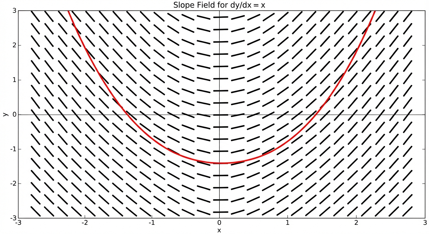
A slope field (or direction field) gives us a graphical representation of a differential equation without solving it algebraically. It draws tiny line segments representing the slope (tangent line) at various points $(x,y)$ on the coordinate plane.
- The differential equation $\frac{dy}{dx} = f(x,y)$ tells you the slope at any specific point.
- Key Concept: The slope field shows the "flow" of the solution curves. A solution curve must follow the path charted by the line segments.
Drawing Slope Fields
To construct a slope field on the AP exam:
- Create a small table of values for the given $(x,y)$ coordinates.
- Plug the coordinates into the differential equation to find $\frac{dy}{dx}$.
- Draw a short segment with that slope at that specific point.
Example: Draw the slope field for $\frac{dy}{dx} = x - y$.
- At $(1,1)$, slope = $1 - 1 = 0$ (Horizontal line).
- At $(0,1)$, slope = $0 - 1 = -1$ (Diagonal down).
- At $(2,0)$, slope = $2 - 0 = 2$ (Steep diagonal up).
Matching Slope Fields to Equations
When asked to match a DE to a graph, look for specific patterns:
- Function of $x$ only ($ rac{dy}{dx} = f(x)$): Slopes are identical vertically (columns have the same slope).
- Function of $y$ only ($ rac{dy}{dx} = f(y)$): Slopes are identical horizontally (rows have the same slope).
- Zero Slope Isoclines: Where is the derivative zero? If $\frac{dy}{dx} = x+y$, slopes should be horizontal along the line $y = -x$.
Euler's Method (BC Only)
Conceptual Overview
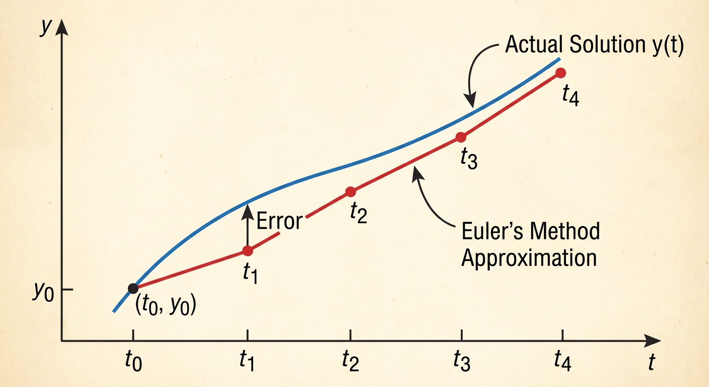
Euler's Method is a numerical approach to approximate the value of a function using its tangent lines. It builds on the idea of local linearity—that close to a point, a function behaves like its tangent line.
The Algorithm
Given $\frac{dy}{dx} = f(x,y)$, an initial point $(x0, y0)$, and a step size $\Delta x$ (or $h$):
Worked Example
Given $\frac{dy}{dx} = 2x + y$, approximate $y(1.2)$ given $y(1) = 3$ with step size $\Delta x = 0.1$.
| Iteration | $x$ | $y$ | Slope ($2x+y$) | $dy = m \cdot \Delta x$ | $y_{new} = y + dy$ |
|---|---|---|---|---|---|
| Start | 1.0 | 3.0 | $2(1)+3 = 5$ | $5(0.1) = 0.5$ | $3.0 + 0.5 = 3.5$ |
| Step 1 | 1.1 | 3.5 | $2(1.1)+3.5 = 5.7$ | $5.7(0.1) = 0.57$ | $3.5 + 0.57 = 4.07$ |
| End | 1.2 | 4.07 |
Answer: $y(1.2) \approx 4.07$.
Critically Important: Euler's method provides an approximation.
- If the curve is concave up, tangent lines lie below the curve, so Euler's method produces an underapproximation.
- If the curve is concave down, tangent lines lie above the curve, so Euler's method produces an overapproximation.
Separation of Variables
This is the primary algebraic method for solving differential equations where variables can be split to opposite sides of the equals sign.
The SIPPY Method
A useful mnemonic to remember the steps for finding a particular solution is SIPPY.
- S - Separate: Algebraically move all $y$ terms (with $dy$) to one side and $x$ terms (with $dx$) to the other.
- I - Integrate: Apply the integral symbol $\int$ to both sides.
- P - Plus C: Immediately add $+C$ to the side with the independent variable (usually $x$). Do not wait until the end.
- P - Plug In: Substitute the initial condition $(x0, y0)$ to solve for the specific value of $C$.
- Y - Y Equals: Algebraically isolate $y$ to write the final general solution $y = f(x)$.
Worked Problem
Solve: $\frac{dy}{dx} = \frac{4x}{y}$ with initial condition $y(0) = 5$.
- Separate: Multiply both sides by $y$ and $dx$.
- Integrate:
- Plus C: Included above.
- Plug In: Use $x=0, y=5$.
Equation so far: $\frac{1}{2}y^2 = 2x^2 + \frac{25}{2}$ - Y Equals:
Multiply by 2: $y^2 = 4x^2 + 25$
Square root: $y = \pm \sqrt{4x^2 + 25}$
Decision: Since $y(0)=5$ (a positive number), we verify the positive root is the correct branch.
Final Answer: $y = \sqrt{4x^2 + 25}$
Exponential Models
Many natural phenomena grow at a rate proportional to their current size (population, radioactive decay, interest).
The Equation
If the rate of change of $y$ is proportional to $y$ itself:
The General Solution
The solution to this differential equation is always exponential:
- $C = y(0)$ (The initial amount)
- $k$ = The growth constant (if $k>0$) or decay constant (if $k<0$).
Logistic Growth (BC Only)
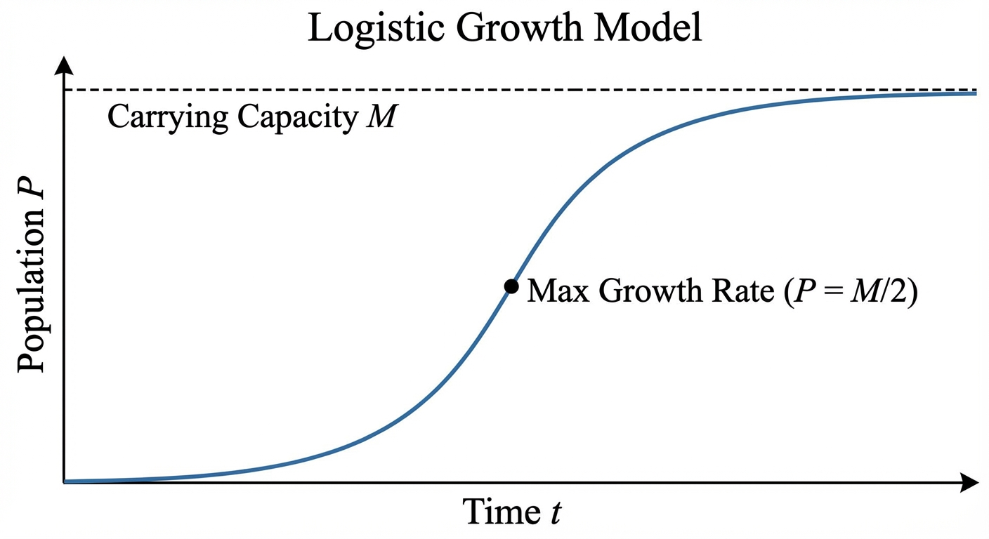
Exponential growth assumes unlimited resources. In the real world, populations hit a limit called the Carrying Capacity ($M$ or $L$).
The Logistic Differential Equation
- $k$: Maximum relative growth rate.
- $M$: Carrying capacity.
- $P$: Population size.
Key Analysis Points
- The Limits: $\lim_{t \to \infty} P(t) = M$. The population approaches the carrying capacity over time.
- Fastest Growth: The rate of change $\frac{dP}{dt}$ is at its maximum when the population is exactly half the carrying capacity ($P = \frac{M}{2}$). This corresponds to the inflection point on the graph.
- The Solution: You rarely need to derive this from scratch, but recognizing the form is helpful:
(where $A$ is a constant determined by the initial population).
Common Mistakes & Pitfalls
"Plus C" Placement Mistake:
- Bad: Integrating $\frac{1}{y} dy = k dt$ to get $\ln|y| = kt$, then solving for $y$ to get $y = e^{kt}$, and then adding $C$ ($y = e^{kt} + C$). This is wrong.
- Good: $\ln|y| = kt + C \rightarrow y = e^{kt+C} \rightarrow y = Ce^{kt}$. The constant of integration affects the coefficient, not the constant term.
Absolute Value Omission:
- When integrating $\int \frac{1}{y} dy$, you MUST write $\ln|y| + C$. Forgetting the absolute value bars can lead to incorrect domain restrictions or missing negative solutions.
Euler's Method Sign Errors:
- Be very careful with positive/negative signs when calculating the new slope at each iteration. A single sign error propagates through the entire remaining table.
Mixing up $\frac{dy}{dx}$ and $\frac{d^2y}{dx^2}$ logic:
- When approximating with tangent lines (Euler's), over/under approximation depends on concavity ($y''$), not whether the function is increasing/decreasing ($y'$).