Unit 6 (AP Calculus BC): Integration and Accumulation of Change — Comprehensive Study Notes
Accumulation of Change: Net Change, Total Change, Signed Area, and Units
Up to this point in calculus, you’ve emphasized the derivative as a rate of change (change per unit). Unit 6 flips that viewpoint: when you know a rate, you can recover the total accumulated change by adding up tiny pieces. That “adding up” process is what an integral does. The integral symbol is often described as the antiderivative idea (undoing a derivative), but it’s also broader than that: a definite integral represents accumulation even when an antiderivative is hard to find.
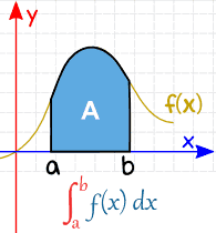
The first type you usually meet is a definite integral, which represents the accumulation of a quantity across an interval and is interpreted geometrically as the signed area between a function and the -axis.
From “rate” to “amount” (why integrals exist)
Suppose you know the velocity of a car %%LATEX1%% in meters per second. Velocity is the rate of change of position: it tells you how many meters of position change happen per second. If you want to know how far the car’s position changes between %%LATEX2%% and , you need to combine (accumulate) all those per-second changes.
Over a very small time interval %%LATEX4%%, the position changes by approximately %%LATEX5%%. Over many small intervals, the total change is approximately the sum of all those little changes. This “add up many small rectangles” idea is the seed of the definite integral.
Net change vs. total change
A big conceptual point on AP questions is that “how much changed” can mean two different things.
Net change includes direction/sign. If the rate is negative, it subtracts from the accumulation.
Total change (total amount) measures the magnitude of change regardless of direction. When a rate can change sign, you typically need absolute value and you often must split the interval.
For velocity:
- Displacement (net change in position) from %%LATEX6%% to %%LATEX7%% is the net accumulation of velocity.
- Total distance traveled is the accumulation of speed, which is .
Signed area as accumulation
Graphically, accumulation is tied to area. If %%LATEX9%% is positive, accumulation adds positive area above the axis. If %%LATEX10%% is negative, the accumulation contributes negative area (it subtracts). That’s why a definite integral naturally matches net change: area below the axis counts negatively.
Units: a built-in reality check
Units help you decide whether you’re computing the right thing. If %%LATEX11%% has units “gallons per minute” and %%LATEX12%% is “minutes,” then a small change is with units gallons. On many FRQs, explicitly stating and checking units is part of a complete justification.
Worked example: net change and total change
A particle has velocity %%LATEX14%% (units: m/s) for %%LATEX15%%.
1) Net change in position (displacement)
An antiderivative is:
Evaluate:
So the net change is meters.
2) Total distance traveled
Distance uses speed %%LATEX20%%. Find where %%LATEX21%%:
So velocity is negative on %%LATEX24%% and positive on %%LATEX25%%.
Compute:
Exam Focus
- Typical question patterns:
- Interpret as a net change in a real situation (motion, flow, growth, temperature change).
- Compare net change vs. total change and explain the difference using a sign change.
- Use units to justify an integral setup.
- Common mistakes:
- Treating a definite integral as “area” without considering sign (below-axis contributes negative).
- Using for total distance when velocity changes sign (you need absolute value and interval splitting).
- Mismatching units (for example integrating a position function to get displacement).
Approximating Accumulation with Riemann Sums (Rectangles, Midpoints, and Tables)
If a definite integral represents accumulation/area under a curve, a natural question is: how do you find that area when the shape is irregular or you only have data? The core idea is to estimate using shapes you do know.
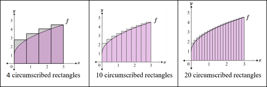
Splitting a region into rectangles produces an approximation, and the more rectangles you use, the better the estimate tends to be (for well-behaved functions). This method is called a Riemann sum.
The rectangle idea (how the approximation is built)
To approximate accumulation of %%LATEX33%% from %%LATEX34%% to :
- Split %%LATEX36%% into %%LATEX37%% subintervals.
- Choose a sample point in each subinterval.
- Approximate the slice by a rectangle with base %%LATEX38%% and height %%LATEX39%%.
- Add all rectangles.
If the partition is equally spaced:
A general Riemann sum is:
This matches the geometry formula “base times height,” repeated and added.
Left, right, and midpoint sums (what changes)
The most common versions differ only by sample point choice:
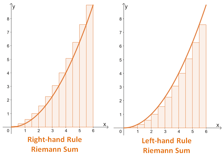
- Left Riemann sum: use left endpoints.
- Right Riemann sum: use right endpoints.
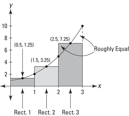
- Midpoint Riemann sum: use midpoints.
If the function is increasing, left sums tend to underestimate and right sums tend to overestimate. If decreasing, the roles reverse.
When data come from a table
Most of the time on AP problems, you’re given values in a table and asked to compute a left, right, midpoint, or trapezoidal approximation. Your job is to identify the widths and which function values correspond to the chosen sample points.
Worked example: midpoint Riemann sum for a function formula
Approximate:
using a midpoint Riemann sum with .
Midpoints: .
Sum inside: , so:
Exact value:
Worked example: Riemann sum from table values (right sum)
Suppose is a rate (liters/min) and you have:
| (min) | 0 | 2 | 4 | 6 | 8 |
|---|---|---|---|---|---|
| 5 | 7 | 6 | 4 | 3 |
Approximate using a right Riemann sum with 4 subintervals.
Right endpoints: .
Interpretation: about 40 liters accumulated.
Worked example: table with unequal subinterval widths (left, right, midpoint idea, and trapezoids)
A common AP-style table:
| 0 | 2 | 4 | 7 |
|---|---|---|---|
| 1 | 6 | 10 | 15 |
Notice the widths are not all the same: from 0 to 2 is width 2, 2 to 4 is width 2, and 4 to 7 is width 3.
- Left sum uses left endpoint heights (do not use the furthest right value):
- Right sum uses right endpoint heights (do not use the furthest left value):
- Midpoint (as shown in many notes) uses a width times a middle height; for instance, a sketchy “midpoint-style” idea might look like:
This is not a complete midpoint sum for the whole interval, but it illustrates the key idea: choose the height at a value in between rather than an endpoint.
- Trapezoidal approximation uses trapezoids on each subinterval:
You do not have to simplify these expressions unless the problem explicitly asks.
Tabular Riemann sums (very common FRQ format)
| Years: | 2 | 3 | 5 | 7 | 10 |
|---|---|---|---|---|---|
| Height: | 1.5 | 2 | 6 | 11 | 15 |
- Trapezoids:
- Left sum:
- Right sum:
Again, you do not have to simplify unless asked.
Exam Focus
- Typical question patterns:
- Build a left/right/midpoint Riemann sum from a table and interpret it as accumulated change.
- Decide whether a left/right sum over- or underestimates based on whether the function is increasing/decreasing.
- Translate a written sum into integral notation or vice versa.
- Common mistakes:
- Using the wrong sample points (for a right sum, accidentally using left endpoints).
- Forgetting the factor or using the wrong width (especially when the table spacing is not uniform).
- Over/underestimate reasoning stated without referencing increasing/decreasing behavior.
The Definite Integral as a Limit (Formal Definition)
Riemann sums are approximations, but calculus makes them exact by taking a limit. This is the formal definition of the definite integral.
What the definite integral means
where %%LATEX68%% and %%LATEX69%% is a sample point in the -th subinterval.
This matters because it tells you what an integral really is: the limit of a sum of many small accumulated changes. The “area under the curve” interpretation is a consequence of this definition.
Notation: sigma form and common index setups
For equal partitions and right endpoints:
For left endpoints:
Midpoints are similar but shifted by half a step.
Why the limit is necessary
With finitely many rectangles, there is error because curves are not rectangles. Sending makes widths tiny, driving that mismatch down for continuous (or piecewise continuous) functions.
Worked example: computing an integral from the definition
Compute:
using the definition with right endpoints.
So the sum equals:
Take the limit:
Exam Focus
- Typical question patterns:
- Write an integral as a limit of a Riemann sum (or the reverse).
- Interpret the meaning of a sum like in context.
- Use properties of sums to evaluate a simple integral from the definition.
- Common mistakes:
- Mixing up and the sample point expression.
- Using wrong bounds for %%LATEX85%% (for right endpoints, %%LATEX86%% to is typical).
- Skipping the meaning of the limit and treating the definition as just “a formula.”
Numerical Integration: Trapezoidal Rule and Simpson’s Rule
Sometimes you can’t (or aren’t supposed to) find an exact antiderivative. Other times you only have a table of values. In these cases, you approximate the definite integral using numerical integration.
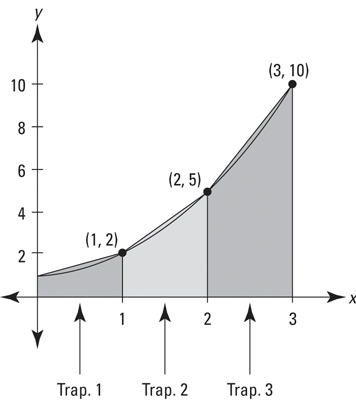
Trapezoidal Rule (better than rectangles for many curves)
The Trapezoidal Rule approximates the region under a curve by trapezoids. Over one subinterval, it’s equivalent to using the trapezoid area formula:
where the “bases” are the function values at the endpoints and the “height” is the width of the interval.
For %%LATEX89%% equal subintervals on %%LATEX90%% with %%LATEX91%% and nodes %%LATEX92%%:
Interior points get coefficient 2 because each is shared by two neighboring trapezoids.
A quick trapezoid example (matching the basic formula idea): if one trapezoid has endpoint heights 2 and 5 and width 1, its area is:
Error intuition: If %%LATEX95%% is concave up, trapezoids tend to sit above the curve so %%LATEX96%% overestimates. If is concave down, it tends to underestimate.
Simpson’s Rule (BC emphasis)
Simpson’s Rule is usually more accurate because it approximates with parabolas over pairs of subintervals. It requires an even number of subintervals .
Coefficients alternate 4 and 2 (4 on odd indices, 2 on even interior indices).
Worked example: Trapezoidal Rule from table data
Using the table below, approximate with the trapezoidal rule.
| 0 | 2 | 4 | 6 | 8 | |
|---|---|---|---|---|---|
| 5 | 7 | 6 | 4 | 3 |
Here %%LATEX103%% and %%LATEX104%%.
Worked example: Simpson’s Rule
Approximate:
using Simpson’s Rule with .
Points: .
On the AP exam, you’d use a calculator for the sine values; the main skill is setting up coefficients correctly.
Exam Focus
- Typical question patterns:
- Compute %%LATEX112%% or %%LATEX113%% from a table (extremely common on FRQs).
- Compare approximations and decide which should be larger using concavity.
- Use a numerical approximation as a step inside a larger modeling problem (accumulation, average value, etc.).
- Common mistakes:
- Forgetting Simpson’s Rule requires even .
- Misplacing the 4 and 2 coefficients in Simpson’s Rule.
- Using incorrectly when the table spacing isn’t 1, or assuming equal spacing when it isn’t.
The Fundamental Theorem of Calculus (Part 1): Accumulation Functions
An accumulation function is defined by an integral with a variable limit:
This means: start at %%LATEX117%%, accumulate values of %%LATEX118%% as %%LATEX119%% moves to %%LATEX120%%, and call the accumulated total .
Statement (FTC Part 1)
If %%LATEX122%% and %%LATEX123%% is continuous, then:
Conceptually, increasing %%LATEX125%% by a tiny amount adds a thin slice of area near %%LATEX126%%, approximately %%LATEX127%%, so the instantaneous rate of change of the accumulated total is %%LATEX128%%.
Chain rule version (upper and lower variable limits)
If:
then:
If the variable limit is on the bottom:
rewrite:
so:
Accumulation functions and graphs: increasing/decreasing and concavity
If:
then:
So %%LATEX136%% increases where %%LATEX137%% is positive and decreases where is negative.
Also:
So %%LATEX140%% is concave up where %%LATEX141%% is increasing, and concave down where is decreasing.
Worked example: basic accumulation derivative
Worked example: chain rule with variable upper limit
Worked example: understanding an accumulation function numerically
If %%LATEX147%% and the graph of %%LATEX148%% is above the axis on %%LATEX149%% and below on %%LATEX150%%, then %%LATEX151%% increases on %%LATEX152%% and decreases on %%LATEX153%%. Maxima occur where %%LATEX154%% with a sign change from positive to negative.
Exam Focus
- Typical question patterns:
- Differentiate an accumulation function defined by an integral (including chain rule upper limits).
- Given a graph/table of %%LATEX155%%, analyze where %%LATEX156%% is increasing/decreasing and concave up/down.
- Find extreme values of an accumulation function using zeros and sign changes of .
- Common mistakes:
- Forgetting the chain rule multiplier when the limit is .
- Confusing the integrand variable %%LATEX159%% with the outside variable %%LATEX160%%.
- Treating %%LATEX161%% like an indefinite integral with %%LATEX162%% (definite integrals do not include ).
The Fundamental Theorem of Calculus (Part 2): Evaluating Definite Integrals with Antiderivatives
A definite (bounded) integral is indicated by having two numbers on the integral sign. Those bounds tell you the interval of accumulation.
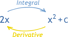
Antiderivatives and the indefinite integral
An antiderivative of %%LATEX164%% is a function %%LATEX165%% such that:
The indefinite integral notation means the family of all antiderivatives:
The constant is called the constant of integration, and it matters because derivatives erase constants.
Core antiderivative idea (power rule “in reverse”)
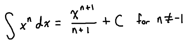
Early in integration, many problems are designed so you can use the power rule pattern. If the derivative power rule multiplies down and decreases the power, then the matching antiderivative pattern increases the power and divides.
For :
A quick simplification example that often appears in notes: integrating can be viewed as:
If an integrand is not immediately in a usable form, algebraically manipulate it so you can apply known rules.
Key trig/exponential antiderivatives (commonly used)
A major speed tip for AP is to know trig derivatives so you can reverse them for integrals:
FTC Part 2 (Evaluation Theorem)
This is sometimes informally called “the (first) fundamental theorem” in some course notes: it’s the rule that lets you evaluate a definite integral using an antiderivative.
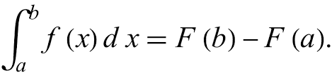
If %%LATEX176%% on %%LATEX177%%, then:
Notation you’ll see:
Worked example: evaluating a definite integral
Compute:
Antiderivative:
Evaluate:
Interpretation: net signed area cancels.
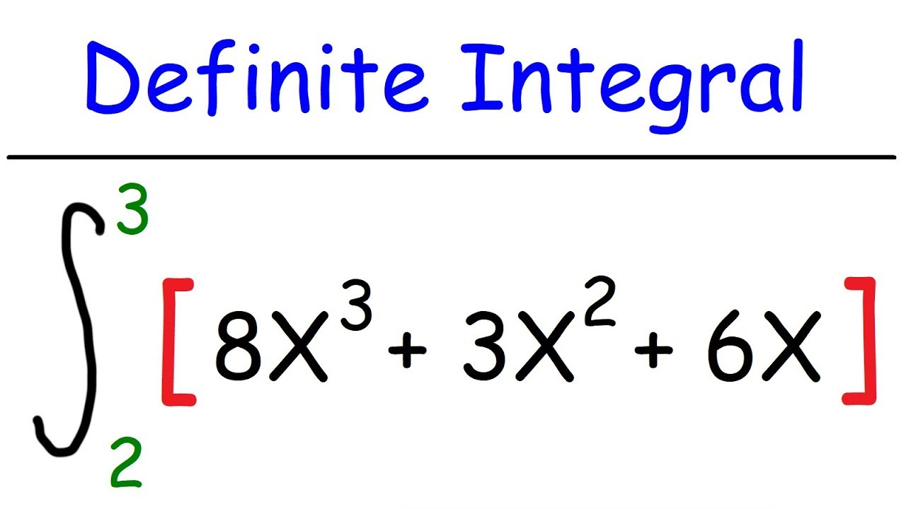
Worked example (from a common FTC demonstration)
Evaluate:
An antiderivative is , so:
Accumulation with an initial condition (common modeling form)
If you know %%LATEX186%% and %%LATEX187%%, then:
This defines even when you cannot find a simple elementary antiderivative.
Worked example: building a function from a derivative
Suppose %%LATEX190%% and %%LATEX191%%. Express exactly.
Exam Focus
- Typical question patterns:
- Evaluate definite integrals using antiderivatives and correct bounds substitution.
- Use FTC to connect a derivative to an accumulation expression, especially with an initial condition.
- Interpret a definite integral as net change and explain sign/cancellation.
- Common mistakes:
- Adding when evaluating a definite integral.
- Evaluating in the wrong order.
- Confusing indefinite and definite integrals (mixing bounds with ).
Properties of Definite Integrals (and How to Use Them Strategically)
Definite integrals come with algebra-like properties that let you simplify problems without computing everything from scratch.
Additivity over intervals
If :
Reversing bounds changes the sign
Integral of a constant
Linearity
Comparison property
If %%LATEX203%% on %%LATEX204%%, then:
Symmetry: even and odd functions
If is even:
If is odd:
Worked example: using linearity with given integral values
Given:
Find:
Worked example: symmetry shortcut
Compute:
The integrand is odd, so:
Exam Focus
- Typical question patterns:
- Use properties to compute a new integral from known integral values.
- Split an integral across a point or combine integrals across adjacent intervals.
- Use even/odd symmetry on to simplify.
- Common mistakes:
- Forgetting that reversing bounds changes the sign.
- Misidentifying even vs odd functions.
- Applying symmetry rules on intervals that are not symmetric about 0.
Average Value of a Function and the Mean Value Theorem for Integrals
Integrals don’t just measure total accumulation; they also help you describe “typical” values over an interval.
Average value of a function
The average value of %%LATEX218%% on %%LATEX219%% is:
Geometrically, this is the height of a rectangle with base %%LATEX221%% that has the same signed area as the region under %%LATEX222%%.
Why average value matters in applications
If is velocity, average value gives average velocity (net displacement divided by time). Be careful: average value of velocity is not average speed unless velocity stays nonnegative.
Worked example: average value
Find the average value of %%LATEX224%% on %%LATEX225%%.
Mean Value Theorem for Integrals
If %%LATEX228%% is continuous on %%LATEX229%%, then there exists at least one %%LATEX230%% in %%LATEX231%% such that:
This guarantees the function actually attains its average value somewhere in the interval.
Worked example: using MVT for integrals
Let %%LATEX233%% be continuous on %%LATEX234%% and suppose:
Average value:
So there exists some %%LATEX237%% in %%LATEX238%% such that:
Exam Focus
- Typical question patterns:
- Compute average value and interpret in context.
- Use the Mean Value Theorem for Integrals to justify that a point %%LATEX240%% exists (and sometimes solve for %%LATEX241%% when is explicit).
- Compare average value of velocity vs average speed.
- Common mistakes:
- Forgetting to divide by .
- Claiming a specific without enough information.
- Using MVT for integrals without stating continuity when justification is required.
Advanced Integration Techniques: Trig Antiderivatives and U-Substitution
Sometimes, getting an integral into a straightforward power-rule form is difficult or essentially impossible with basic algebra alone. In those cases, you use other techniques.
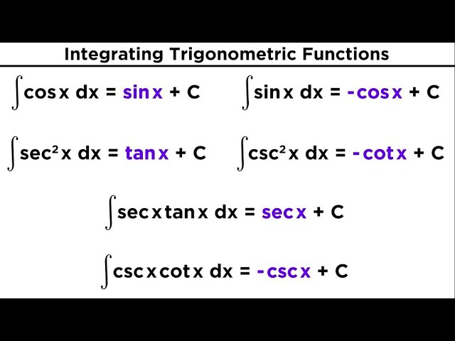
Trigonometric integrals (memorization strategy)
If your integral contains trigonometry, it’s often fastest on a timed AP exam to rely on memorized derivative-antiderivative pairs. For example, since:
it follows that:
You can derive these relationships, but efficiency matters.
U-substitution (substitution method)
U-substitution is a structured way to reverse the chain rule.
A standard process:
- Choose a term to be your .
- Differentiate to find .
- Rewrite %%LATEX249%% in terms of %%LATEX250%% and substitute into the integral.
- Integrate with respect to .
- Substitute back in terms of the original variable.
U-substitution can be tricky at first but very helpful.
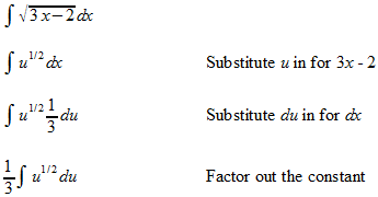
Worked example: u-substitution
Evaluate:
Let:
Then:
So:
Substitute:
Back-substitute:
Exam Focus
- Typical question patterns:
- Recognize when a substitution like simplifies an integrand with a “inside function” power.
- Use memorized trig antiderivatives quickly in definite-integral evaluation.
- Common mistakes:
- Choosing %%LATEX259%% but not correctly converting %%LATEX260%% (forgetting the derivative factor).
- Integrating in terms of but forgetting to substitute back.
- Treating substitution as optional when the integrand is not in a directly integrable form.