AP Calculus AB Unit 6: Integration as Accumulation (Riemann Sums, FTC, Numerical Methods, Substitution, and Symmetry)

Accumulation and the Net Change Idea

Calculus often starts with a very practical problem: you can measure or model a rate of change, but what you really want is a total amount. The integral is the tool that turns “change per unit” into “total change,” so it is deeply connected to both accumulation and (in many settings) area under a curve.

For example:

• You might know a car’s velocity (rate of change of position), but you want displacement (how far the car traveled, with direction).
• You might know the flow rate of water into a tank (gallons per minute), but you want the total volume added over a time interval.

This is the central theme of integration: accumulation.

From “rate” to “total change”

If a quantity %%LATEX0%% changes over time %%LATEX1%%, then its rate of change is %%LATEX2%% (also written %%LATEX3%%). Conceptually, %%LATEX4%% tells you how fast %%LATEX5%% is changing right now, and the accumulated change in %%LATEX6%% from %%LATEX7%% to t=b should be the “sum” of all those tiny changes.

If you approximate time using small subintervals, then over a short time step %%LATEX9%% near time %%LATEX10%%, the change in Q is approximately:

\Delta Q \approx Q'(t)\Delta t

If you add these approximate changes over many subintervals, you get an approximation for total change. When you let the subintervals get extremely small, that approximation becomes exact. That “limit of sums” is what we call a definite integral.

Definite integrals, area under a curve, and accumulation

A definite integral (a “bounded integral”) is written:

\int_a^b f(x)\,dx

In many AP Calculus AB problems, this value represents the signed area between the graph of %%LATEX14%% and the %%LATEX15%%-axis on [a,b]. Even when you don’t have a simple formula for the region (or even a formula for the function), you can still estimate the region using shapes you do know.

Reference sketches from the original notes:

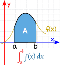
The key idea is that more rectangles/trapezoids typically means a better estimate.

Net change versus total change

A key idea in AP Calculus AB is that integrals naturally represent net change.

• Net change accounts for increases and decreases with sign.
  • If a rate is positive, the quantity is increasing.
  • If a rate is negative, the quantity is decreasing.

For motion:

• If v(t) > 0, you move in the positive direction.
• If v(t) < 0, you move in the negative direction.

So the accumulated change in position (displacement) over [a,b] is net change.

The Net Change Theorem (conceptual form)

If %%LATEX20%% on an interval, then the total change in %%LATEX21%% from %%LATEX22%% to %%LATEX23%% is the integral of its rate of change:

F(b)-F(a)=\int_a^b f(x)\,dx

This statement is one of the most important meaning statements in the course: integrals turn rates into accumulated change.

Units (a reliable way to check your work)

Units are a powerful reality check:

• If %%LATEX25%% is in “gallons per minute” and %%LATEX26%% is in minutes, then %%LATEX27%% has units “gallons,” and %%LATEX28%% has units “gallons.”
• If %%LATEX29%% is in “meters per second” and %%LATEX30%% is in seconds, then \int v(t)\,dt is in meters.

If your final units don’t make sense, your setup is probably wrong.

Worked example: displacement from velocity

Suppose a particle has velocity %%LATEX32%% (meters per second) for %%LATEX33%%.

What this means: the position function %%LATEX34%% satisfies %%LATEX35%%.

Net change in position (displacement):

s(2)-s(0)=\int_0^2 (3t^2-4)\,dt

Compute:

\int_0^2 (3t^2-4)\,dt=\left[t^3-4t\right]_0^2=(8-8)-(0-0)=0

So the displacement is 0 meters. This does not mean the particle didn’t move; it means it ended where it started (it moved forward and backward with net zero).

Worked example: volume added from flow rate

Water flows into a tank at rate %%LATEX39%% gallons per minute for %%LATEX40%%.

Total volume added:

\int_0^{\pi} (5+2\sin(t))\,dt=\left[5t-2\cos(t)\right]_0^{\pi}=(5\pi-2\cos(\pi))-(0-2\cos(0))

=5\pi-2(-1)+2(1)=5\pi+4

Exam Focus

Typical question patterns:

• You’re given a rate function (or a table of rates) and asked for total change over an interval.
• Motion context: interpret displacement vs distance traveled.
• Unit analysis: explain what an integral represents in words and units.
• “Area under the curve” interpretation, especially when you only have a graph or data.

Common mistakes:

• Treating net change as “total amount” even when the rate becomes negative.
• Forgetting that integrals accumulate with sign, so “ending where you started” can still involve lots of movement.
• Ignoring units, leading to incorrect interpretation of what the integral measures.

Approximating Accumulation with Riemann Sums

Before you can compute integrals exactly, you need to understand how integrals are built: by adding up lots of small contributions. When the shape under a curve is not something you have a direct formula for, you estimate it using rectangles (and later trapezoids).

Partitioning an interval

To accumulate a rate or to approximate area, you break the interval %%LATEX43%% into %%LATEX44%% subintervals.

If the partition is equal-width, then each subinterval has width:

\Delta x=\frac{b-a}{n}

The endpoints are:

x_0=a,\;x_1=a+\Delta x,\;\dots,\;x_n=b

Rectangles: the core approximation idea

Suppose you have a function %%LATEX47%%. Over a small subinterval, %%LATEX48%% doesn’t change much, so you approximate it by a constant value.

Pick a sample point %%LATEX49%% in each subinterval %%LATEX50%%. Then approximate the contribution on that subinterval by a rectangle:

• height f(x_i^*)
• width \Delta x

Area (or accumulated amount) from that subinterval is approximately:

f(x_i^*)\Delta x

Add all rectangles:

\sum_{i=1}^n f(x_i^*)\Delta x

This is a Riemann sum. The rectangle idea is always “base times height,” so each rectangle contributes:

\text{area} \approx (\text{width})(\text{height})

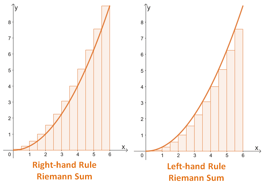
Common choices of sample points

• Left Riemann sum: x_i^*=x_{i-1} (use the left endpoint)
• Right Riemann sum: x_i^*=x_i (use the right endpoint)
• Midpoint Riemann sum: x_i^*=\frac{x_{i-1}+x_i}{2} (use the midpoint)

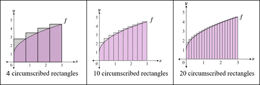
As you increase n (more rectangles), the approximation typically improves.

Reference sketch from the original notes:

Definite integral as a limit of Riemann sums

The definite integral is defined as the limit of Riemann sums as the partition gets infinitely fine:

\int_a^b f(x)\,dx=\lim_{n\to\infty}\sum_{i=1}^n f(x_i^*)\Delta x

This definition matters because:

• It explains what an integral means (accumulation, not just an “antiderivative trick”).
• It allows you to approximate integrals even when you can’t integrate symbolically.

Signed area: why integrals can be negative

If %%LATEX61%% is below the %%LATEX62%%-axis, then rectangle heights are negative, so the integral adds negative contributions. That’s why \int_a^b f(x)\,dx is signed area (area above the axis minus area below).

If you want total area between the graph and the axis, you generally need an absolute value (this idea becomes central in applications of integration).

Worked example: left and right sums from a table (equal spacing)

Suppose %%LATEX64%% is measured at equally spaced points from %%LATEX65%% to %%LATEX66%% with %%LATEX67%%:

Left sum on [0,4] with 4 subintervals:

L_4=\Delta x\left(f(0)+f(1)+f(2)+f(3)\right)

L_4=1(2+5+4+6)=17

Right sum:

R_4=\Delta x\left(f(1)+f(2)+f(3)+f(4)\right)

R_4=1(5+4+6+3)=18

Interpretation: %%LATEX75%% is approximately between %%LATEX76%% and 18.

Worked example: writing a Riemann sum expression

Write a Riemann sum for %%LATEX78%% using %%LATEX79%% equal subintervals and right endpoints.

Step 1: compute width

\Delta x=\frac{3-1}{n}=\frac{2}{n}

Step 2: right endpoints

x_i=1+i\Delta x=1+\frac{2i}{n}

Step 3: sum

\sum_{i=1}^n f(x_i)\Delta x=\sum_{i=1}^n \left(1+\frac{2i}{n}\right)^2\frac{2}{n}

You are usually not asked to take the limit by hand in AP Calculus AB, but you should be comfortable building this expression.

Table-based Riemann sums when widths are not equal (include the widths!)

On the AP exam, you are often given a table where the %%LATEX83%%-values are not equally spaced. In that situation, each rectangle’s width is the change in %%LATEX84%% for that interval.

Example table (as given in the original notes):

Here the widths are %%LATEX87%%, %%LATEX88%%, and 3.

• Left sum (use left endpoints, so do not use the furthest right value 15):

2\cdot 1+2\cdot 6+3\cdot 10

• Right sum (use right endpoints, so do not use the furthest left value 1):

2\cdot 6+2\cdot 10+3\cdot 15

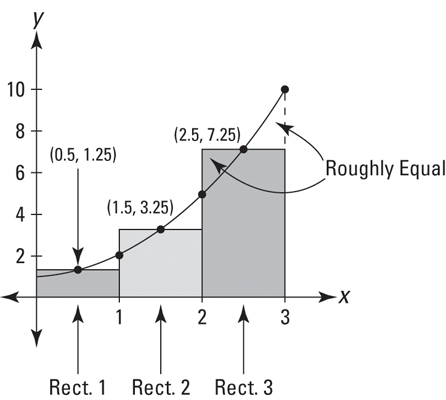
• Midpoint idea (as shown in the original notes, not fully expanded):

4\cdot 6

This expression is illustrating the midpoint concept: use a “middle” height on an interval. (When you do an actual midpoint sum from a table, you must be careful about what midpoints you have data for and whether the subintervals are equal.)

Reference sketch from the original notes:

Exam Focus

Typical question patterns:

• “Write the Riemann sum that represents \int_a^b f(x)\,dx using right endpoints/midpoints.”
• Approximate an integral from a table using left/right/midpoint sums.
• Use a table with unequal subinterval widths (you must multiply each height by its own width).
• Conceptual: explain why increasing n improves the approximation.

Common mistakes:

• Mixing up left vs right endpoints (using the wrong table entries).
• Incorrect \Delta x when the interval length is not 1, or assuming widths are equal when they are not.
• Forgetting that integrals represent signed accumulation; negative values reduce the total.

Definite Integral Notation and Core Properties

Once you accept that integrals measure accumulation, you need a symbolic language for working with them. The notation also encodes important meaning.

Anatomy of a definite integral

A definite integral looks like:

\int_a^b f(x)\,dx

• \int is the integral sign (think “sum of infinitely many tiny pieces”).
• %%LATEX100%% and %%LATEX101%% are the limits of integration.
• f(x) is the integrand, the quantity being accumulated.
• dx indicates the variable of integration and hints at the tiny width of each slice.

A common misconception is that dx is “just decoration.” In fact, it matters for substitution and for interpreting units.

Notation equivalences you should recognize

Sometimes the variable name changes. That does not change the value as long as it’s used consistently:

\int_a^b f(x)\,dx=\int_a^b f(t)\,dt

Quick reference of equivalent forms:

Key properties (with meaning)

These properties let you simplify integrals without finding an antiderivative.

1) Reversing limits changes the sign

\int_a^b f(x)\,dx=-\int_b^a f(x)\,dx

2) Integral over a zero-length interval is zero

\int_a^a f(x)\,dx=0

3) Additivity over intervals

\int_a^b f(x)\,dx=\int_a^c f(x)\,dx+\int_c^b f(x)\,dx

4) Linearity (add and scale inside integrals)

\int_a^b (f(x)+g(x))\,dx=\int_a^b f(x)\,dx+\int_a^b g(x)\,dx

\int_a^b (k f(x))\,dx=k\int_a^b f(x)\,dx

5) Comparison property (ordering)
If %%LATEX115%% on %%LATEX116%%, then:

\int_a^b f(x)\,dx\ge\int_a^b g(x)\,dx

Worked example: using properties with given values

Suppose you are told:

\int_0^2 f(x)\,dx=5

\int_0^2 g(x)\,dx=-1

Find \int_0^2 (3f(x)-2g(x))\,dx.

Use linearity:

\int_0^2 (3f(x)-2g(x))\,dx=3\int_0^2 f(x)\,dx-2\int_0^2 g(x)\,dx

Substitute values:

=3(5)-2(-1)=15+2=17

Worked example: splitting intervals

Given %%LATEX123%% and %%LATEX124%%, find \int_3^5 f(x)\,dx.

By additivity:

\int_1^5 f(x)\,dx=\int_1^3 f(x)\,dx+\int_3^5 f(x)\,dx

So:

12=4+\int_3^5 f(x)\,dx

\int_3^5 f(x)\,dx=8

Exam Focus

Typical question patterns:

• Compute a new integral using properties from a set of given integrals.
• Split or combine integrals across adjacent intervals.
• Conceptual comparisons: decide which integral is larger based on graphs or inequalities.

Common mistakes:

• Forgetting the negative when reversing limits.
• Distributing incorrectly across different limits (linearity works when the limits match).
• Splitting incorrectly at c (using mismatched endpoints).

The Fundamental Theorem of Calculus (Part 1) and Accumulation Functions

The definite integral is defined using limits of sums. That definition is conceptually powerful, but it’s not always convenient for computation.

The Fundamental Theorem of Calculus (FTC) is the bridge between:

• integrals as accumulation (geometry and sums)
• derivatives and antiderivatives (algebraic computation)

Accumulation functions

An accumulation function is built by integrating up to a variable endpoint:

A(x)=\int_a^x f(t)\,dt

Here %%LATEX131%% is a dummy variable. Interpretation: %%LATEX132%% is “the accumulated amount of %%LATEX133%% from %%LATEX134%% to x.”

FTC Part 1 (derivative of an integral)

If f is continuous, then:

\frac{d}{dx}\left(\int_a^x f(t)\,dt\right)=f(x)

Intuition: moving the upper limit from %%LATEX138%% to %%LATEX139%% adds a thin slice of area with approximate area %%LATEX140%%, so dividing by %%LATEX141%% and taking the limit gives f(x).

A more general form: variable upper limit plus chain rule

\frac{d}{dx}\left(\int_a^{g(x)} f(t)\,dt\right)=f(g(x))g'(x)

Worked example: differentiating an accumulation function

Let:

H(x)=\int_2^x \sqrt{1+t^4}\,dt

Then:

H'(x)=\sqrt{1+x^4}

Worked example: chain rule with variable limit

Let:

P(x)=\int_0^{x^2} \cos(t)\,dt

Differentiate:

P'(x)=\cos(x^2)\cdot 2x

Exam Focus

Typical question patterns:

• Differentiate an expression containing an integral with variable limit(s).
• Use the derivative of an accumulation function to evaluate a derivative at a point.
• Interpret \frac{d}{dx}\left(\int_a^x f(t)\,dt\right) conceptually.

Common mistakes:

• Trying to compute an antiderivative when the question is asking for a derivative (FTC Part 1 situation).
• Forgetting to multiply by %%LATEX149%% when the upper limit is %%LATEX150%%.
• Leaving the dummy variable (like t) in the final answer.

Reading Accumulation Functions: Increasing/Decreasing, Extrema, and Concavity

FTC Part 1 gives you a derivative quickly, so you can analyze an accumulation function’s behavior using derivative reasoning.

Let:

A(x)=\int_a^x f(t)\,dt

Then:

A'(x)=f(x)

Increasing and decreasing

Because A'(x)=f(x):

• %%LATEX155%% is increasing where %%LATEX156%%.
• %%LATEX157%% is decreasing where %%LATEX158%%.

Local maxima and minima

A local extremum of %%LATEX159%% occurs where %%LATEX160%% and changes sign.

Since A'(x)=f(x):

• candidates are where f(x)=0
• positive to negative gives a local maximum of A
• negative to positive gives a local minimum of A

Concavity

Differentiate again:

A''(x)=f'(x)

So:

• %%LATEX166%% is concave up where %%LATEX167%% (where f is increasing).
• %%LATEX169%% is concave down where %%LATEX170%% (where f is decreasing).

Connecting to motion (helpful analogy)

If %%LATEX172%% is position and %%LATEX173%% is velocity, then:

s(t)=s(a)+\int_a^t v(u)\,du

Worked example: behavior from a sign chart

Suppose f(x) has the following sign behavior:

• %%LATEX176%% on %%LATEX177%%
• %%LATEX178%% on %%LATEX179%%
• %%LATEX180%% on %%LATEX181%%

For A(x)=\int_0^x f(t)\,dt:

• %%LATEX183%% increases on %%LATEX184%%
• %%LATEX185%% decreases on %%LATEX186%%
• %%LATEX187%% increases on %%LATEX188%%

So %%LATEX189%% has a local maximum at %%LATEX190%% and a local minimum at x=4.

Worked example: using a graph-based idea (no computation)

If you are given that %%LATEX192%% is increasing on %%LATEX193%%, then for A(x)=\int_0^x f(t)\,dt:

• %%LATEX195%% on %%LATEX196%%
• so %%LATEX197%% is concave up on %%LATEX198%%.

Exam Focus

Typical question patterns:

• Given a graph of %%LATEX199%%, determine where %%LATEX200%% is increasing/decreasing.
• Identify where %%LATEX201%% has local extrema based on where %%LATEX202%% crosses the axis.
• Determine concavity of %%LATEX203%% from where %%LATEX204%% is increasing/decreasing.

Common mistakes:

• Treating %%LATEX205%% like it has the same graph as %%LATEX206%% (they are related by derivative, not equal).
• Claiming %%LATEX207%% has an extremum whenever %%LATEX208%% without checking for a sign change.
• Mixing up concavity: concavity of %%LATEX209%% depends on %%LATEX210%%, not directly on the sign of f.

Antiderivatives and the Fundamental Theorem of Calculus (Part 2)

FTC Part 1 tells you how to differentiate integrals. FTC Part 2 tells you how to evaluate definite integrals using antiderivatives (this was called the “first fundamental theorem” in the original notes, but it is most commonly presented in class as FTC Part 2 / the Evaluation Theorem).

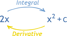
Antiderivatives and indefinite integrals

An antiderivative of %%LATEX212%% is a function %%LATEX213%% such that:

F'(x)=f(x)

The indefinite integral notation represents the family of all antiderivatives:

\int f(x)\,dx=F(x)+C

The %%LATEX216%% is very important. Since the derivative of any constant is %%LATEX217%%, reversing differentiation cannot recover which constant was there, so we include the constant of integration.

A common misconception is to treat \int f(x)\,dx as a number. Without limits, it is a family of functions.

Power rule for antiderivatives (the main workhorse)

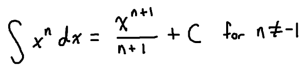
For many algebraic integrals in AP Calculus AB, you primarily use the reverse of the power rule. If taking a derivative means “multiply down and decrease the exponent,” then antidifferentiating means “divide and increase the exponent.”

In particular, for n\ne -1:

\int x^n\,dx=\frac{x^{n+1}}{n+1}+C

Important practical note from the original notes: if an integrand is not in a direct power-rule form, you often algebraically manipulate it until it is.

Example reminder from the original notes: the integral of 2x is

\int 2x\,dx=\frac{2x^2}{2}+C=x^2+C

Reference image from the original notes:

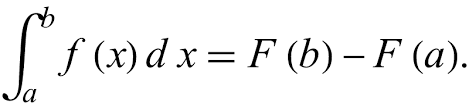
FTC Part 2 (evaluation theorem)

If %%LATEX223%% on an interval containing %%LATEX224%%, then:

\int_a^b f(x)\,dx=F(b)-F(a)

This is what makes integrals computationally practical.

Reference image from the original notes:

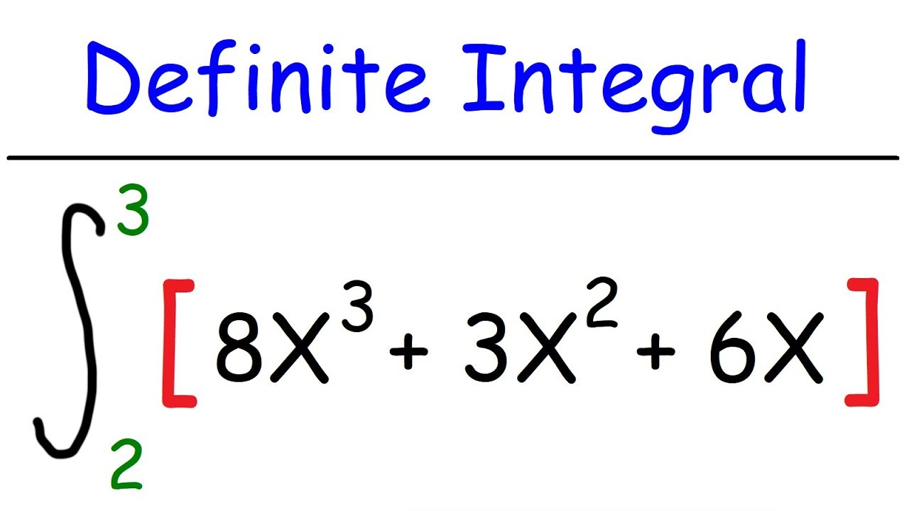
Worked example: a basic definite integral

Evaluate:

\int_1^4 (2x-3)\,dx

Step 1: antiderivative

\int (2x-3)\,dx=x^2-3x+C

Step 2: apply bounds

\int_1^4 (2x-3)\,dx=\left[x^2-3x\right]_1^4=(16-12)-(1-3)=4-(-2)=6

Worked example: using FTC with a provided antiderivative

Suppose %%LATEX229%% and you are given %%LATEX230%%. Find:

\int_2^5 \ln(x)\,dx

By FTC Part 2:

\int_2^5 \ln(x)\,dx=F(5)-F(2)=F(5)-1

You cannot simplify further without more information about F(5) or an explicit formula.

Worked example: definite integral using the evaluation idea (from the original notes)

For %%LATEX234%% on %%LATEX235%%, an antiderivative is x^2, so:

\int_2^3 2x\,dx=3^2-2^2

Exam Focus

Typical question patterns:

• Evaluate a definite integral by finding an antiderivative and using F(b)-F(a).
• Use given information about an antiderivative (values of F) to compute a definite integral.
• Recognize that the numbers on the integral indicate a definite (bounded) integral.
• Remembering +C on indefinite integrals.

Common mistakes:

• Forgetting to evaluate at both bounds (only plugging in b).
• Dropping parentheses when subtracting: F(b)-F(a) must be handled carefully.
• Confusing indefinite and definite integrals (adding +C to a definite integral result).
• Failing to manipulate algebraically into a power-rule-friendly form when appropriate.

Numerical Integration: Midpoint, Trapezoidal Rule, and Error Direction

Sometimes you can’t find an antiderivative easily, or you’re given data in a table instead of a formula. In those cases, you approximate integrals numerically using rectangles (midpoint) or trapezoids.

When numerical methods are used

You use numerical integration when:

• f(x) has no elementary antiderivative.
• You only have sampled values (experimental data).
• You need an approximate value quickly.

AP Calculus AB emphasizes setting up and applying these methods correctly, and interpreting whether an approximation is an overestimate or underestimate in common situations.

Midpoint rule (as a Riemann sum)

On %%LATEX245%% with %%LATEX246%% equal subintervals and \Delta x=\frac{b-a}{n}, the midpoint rule approximation is:

M_n=\Delta x\sum_{i=1}^n f\left(\frac{x_{i-1}+x_i}{2}\right)

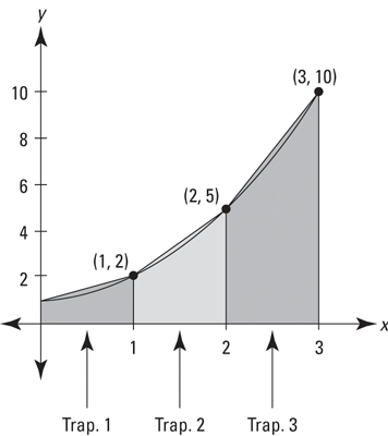
Trapezoidal rule (averaging left and right)

The trapezoidal rule approximates the region under the curve by trapezoids instead of rectangles.

Geometric trapezoid area reminder from the original notes: if the parallel bases have lengths %%LATEX249%% and %%LATEX250%% and the height is h, then

\text{Area}=\frac{1}{2}(b_1+b_2)h

So, for example (as stated in the original notes), if an interval has width %%LATEX253%% and the endpoint heights are %%LATEX254%% and 5, then that trapezoid’s area is

\frac{1}{2}(2+5)(1)

With n equal subintervals, trapezoidal rule is commonly written as:

T_n=\frac{\Delta x}{2}\left(f(x_0)+2f(x_1)+2f(x_2)+\cdots+2f(x_{n-1})+f(x_n)\right)

A helpful way to remember why the middle terms get doubled: each interior point is used as the right endpoint of one trapezoid and the left endpoint of the next.

Reference sketches from the original notes:

Estimating overestimate vs underestimate (qualitative)

Two common facts:

• If f is increasing, then left sums tend to underestimate and right sums tend to overestimate.
• For the trapezoidal rule, concavity matters:
  • If %%LATEX260%% is concave up, trapezoids tend to lie above the curve, so %%LATEX261%% is often an overestimate.
  • If %%LATEX262%% is concave down, %%LATEX263%% is often an underestimate.

Worked example: trapezoidal rule from a table

Approximate \int_0^4 f(x)\,dx using the trapezoidal rule given values:

Here %%LATEX267%% and %%LATEX268%%.

Apply trapezoidal rule:

T_4=\frac{1}{2}\left(f(0)+2f(1)+2f(2)+2f(3)+f(4)\right)

T_4=\frac{1}{2}\left(2+2\cdot 5+2\cdot 4+2\cdot 6+3\right)

=\frac{1}{2}(2+10+8+12+3)=\frac{35}{2}=17.5

Worked example: midpoint rule from a formula

Approximate %%LATEX272%% with %%LATEX273%% using midpoint rule.

Step 1: width

\Delta x=\frac{2-0}{2}=1

Subintervals are %%LATEX275%% and %%LATEX276%%. Midpoints are %%LATEX277%% and %%LATEX278%%.

So:

M_2=1\left(f(0.5)+f(1.5)\right)=0.5^2+1.5^2=0.25+2.25=2.5

The exact value is:

\int_0^2 x^2\,dx=\left[\frac{x^3}{3}\right]_0^2=\frac{8}{3}

So %%LATEX281%% is slightly below %%LATEX282%%.

Tabular trapezoids/left/right sums you may leave unsimplified

Original note emphasis: on many AP free-response problems, you do not have to simplify the final numeric approximation expression if the setup is correct.

Example (as given):

• Trapezoids:

\frac{1}{2}(1.5+2)(1)+\frac{1}{2}(2+6)(2)+\frac{1}{2}(6+11)(2)+\frac{1}{2}(11+15)(3)

• Left sum:

1\cdot 1.5+2\cdot 2+2\cdot 6+3\cdot 11

• Right sum:

1\cdot 2+2\cdot 6+2\cdot 11+3\cdot 15

Exam Focus

Typical question patterns:

• Use trapezoidal rule to approximate an integral from a table of values.
• Use left/right/midpoint sums with specified n on a given interval.
• Decide whether an approximation is an overestimate or underestimate based on increasing/decreasing and concavity.
• Set up (and sometimes leave) numerical expressions from a table without simplifying.

Common mistakes:

• Forgetting the factor \Delta x or using the wrong widths from a non-uniform table.
• In trapezoidal rule, forgetting to double the interior terms.
• Making over/under conclusions without checking whether the method depends on monotonicity (left/right) or concavity (trapezoids).

Integration by Substitution (Reverse Chain Rule)

Some integrals are difficult not because you lack antiderivative rules, but because the expression is a composition of functions. Substitution (often called u-substitution) is the technique that undoes the chain rule.

The idea: reverse the chain rule

The chain rule says:

\frac{d}{dx}f(g(x))=f'(g(x))g'(x)

Substitution recognizes the pattern: if your integrand looks like

f'(g(x))g'(x)

then an antiderivative is

f(g(x))+C

The substitution procedure (step-by-step)

When you do u-substitution:
1) Choose a term to be your %%LATEX293%%, usually the “inside” function: %%LATEX294%%.
2) Differentiate to get %%LATEX295%%, which tells you %%LATEX296%%.
3) Substitute your %%LATEX297%% value for the inside expression and your %%LATEX298%% expression for the remaining differential pieces.
4) Take the integral in terms of %%LATEX299%%. 5) Convert back to %%LATEX300%% unless you changed bounds in a definite integral.

U-substitution is tricky but helpful for some problems.

Reference image from the original notes:

Definite integrals: two correct approaches

If you have a definite integral, you can either:

• Substitute, integrate, convert back to x, then apply original bounds.
• Substitute and also change the bounds into u-bounds, then never convert back.

Both are valid, but mixing them (changing bounds and then converting back) is a common source of errors.

Worked example: basic substitution

Evaluate:

\int 2x\cos(x^2)\,dx

Let:

u=x^2

Then:

du=2x\,dx

So the integral becomes:

\int \cos(u)\,du=\sin(u)+C

Substitute back:

\sin(x^2)+C

Worked example: substitution with a definite integral (change bounds)

Evaluate:

\int_0^1 \frac{3x^2}{1+x^3}\,dx

Let:

u=1+x^3

Then:

du=3x^2\,dx

Change bounds:

• when %%LATEX311%%, %%LATEX312%%
• when %%LATEX313%%, %%LATEX314%%

Integral becomes:

\int_1^2 \frac{1}{u}\,du

Compute:

\int_1^2 \frac{1}{u}\,du=\left[\ln(u)\right]_1^2=\ln(2)-\ln(1)=\ln(2)

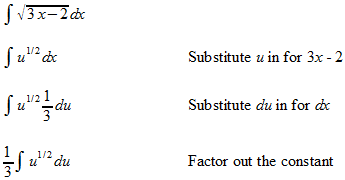
Worked example: u-substitution with a power (from the original notes)

Evaluate:

\int (x-4)^{10}\,dx

Let:

u=x-4

Then:

\frac{du}{dx}=1

So:

dx=\frac{du}{1}

Rewrite and integrate:

\int u^{10}\,du=\frac{u^{11}}{11}+C

Back-substitute:

\frac{(x-4)^{11}}{11}+C

Recognizing common substitution patterns

Substitution is most likely when you see a composition along with (a constant multiple of) its derivative:

• Powers: \int (g(x))^n g'(x)\,dx
• Exponentials: \int e^{g(x)}g'(x)\,dx
• Reciprocals: \int \frac{g'(x)}{g(x)}\,dx
• Trig compositions: %%LATEX326%% and %%LATEX327%%

Exam Focus

Typical question patterns:

• Compute an integral that matches reverse chain rule.
• Definite integral where changing bounds avoids back-substitution.
• Identify an appropriate substitution and explain why it works.

Common mistakes:

• Choosing %%LATEX328%% but not rewriting the entire integral in terms of %%LATEX329%% (leaving stray x factors).
• Incorrect du (especially missing constants).
• Changing bounds and then also converting back to x, causing mismatched limits.

Integrals with Symmetry (Even and Odd Functions)

Symmetry can turn a difficult-looking definite integral into an easy one, especially when the bounds are symmetric around 0.

Even and odd functions

A function is even if:

f(-x)=f(x)

A function is odd if:

f(-x)=-f(x)

Integral shortcuts on symmetric intervals

On [-a,a]:

If f is even, then:

\int_{-a}^a f(x)\,dx=2\int_0^a f(x)\,dx

If f is odd, then:

\int_{-a}^a f(x)\,dx=0

Worked example: even function

Evaluate:

\int_{-3}^3 (x^2+5)\,dx

So:

\int_{-3}^3 (x^2+5)\,dx=2\int_0^3 (x^2+5)\,dx

Compute:

2\left[\frac{x^3}{3}+5x\right]_0^3=2\left(\frac{27}{3}+15\right)=2(9+15)=48

Worked example: odd function

Evaluate:

\int_{-2}^2 (x^3-4x)\,dx

Because the integrand is odd:

\int_{-2}^2 (x^3-4x)\,dx=0

Exam Focus

Typical question patterns:

• Decide whether an integrand is even/odd and simplify an integral over [-a,a].
• Combine symmetry with properties (splitting intervals, linearity).
• Conceptual graph reasoning: explain cancellation for odd functions.

Common mistakes:

• Assuming symmetry applies when the interval is not symmetric around %%LATEX347%% (for example %%LATEX348%%).
• Misclassifying functions: sums of even functions are even; sums of odd functions are odd; even plus odd is neither.
• Forgetting that the “odd integral equals 0” is about signed area, not total area.

Common Antiderivative Patterns (Including Trig) and Timed-Exam Advice

Some integrals are not best handled by forcing power-rule algebra. In AP Calculus AB, you should also recognize basic trig antiderivatives quickly.

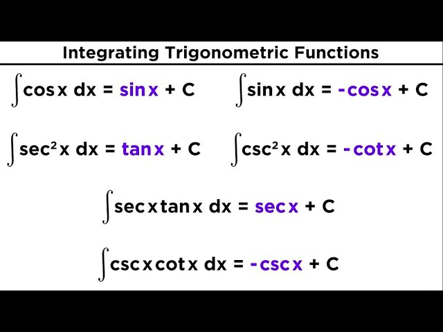
Trig integrals (memorize the matching derivative pairs)

A practical timed-exam tip from the original notes: if your integral contains trigonometry, it is often most efficient to memorize common derivative relationships and reverse them.

Example relationship:

\frac{d}{dx}(\sin(x))=\cos(x)

Therefore:

\int \cos(x)\,dx=\sin(x)+C

(You can derive these, but memorization saves time on the AP exam.)

Reference image from the original notes:

Exam Focus

Typical question patterns:

• Evaluate a basic trig integral by recognizing which derivative it matches.
• Decide quickly whether to use a direct known antiderivative, algebra to power-rule form, or u-substitution.

Common mistakes:

• Forgetting the constant of integration C on indefinite integrals.
• Losing time trying to “re-derive” common trig derivatives during a timed test instead of using memorized pairs.
• Forcing power rule in situations where substitution or a known trig antiderivative is the natural method.