Comprehensive Guide to Production, Cost Analysis, and Perfect Competition
Unit 3: Production, Cost, and the Perfect Competition Model
3.1 The Production Function
Before businesses can assess profit, they must understand the relationship between what they put into a process (inputs) and what they get out (outputs). This relationship is the Production Function.
Key Terms & Time Periods
- Inputs (Factors of Production): Resources used to produce goods and services (Land, Labor, Capital, Entrepreneurship).
- Total Product ($TP$ or $Q$): The total quantity of output produced.
- Marginal Product ($MP$): The additional output generated by adding one more unit of input (usually labor).
- Average Product ($AP$): Output per unit of input.
It is crucial to distinguish between the short run and the long run:
- Short Run: A period where at least one input is fixed (usually Capital, like a factory size or oven) and others are variable (usually Labor/workers).
- Long Run: A period long enough that all inputs can be varied. There are no fixed costs in the long run.
The Law of Diminishing Marginal Returns
This is the foundational concept of short-run production. It states that as you add variable resources (workers) to fixed resources (ovens), the additional output produced from each new worker will eventually fall.
- Stage 1 (Increasing Returns): Specialization allows $MP$ to rise. Total product increases at an increasing rate.
- Stage 2 (Diminishing Returns): Fixed resources get overcrowded. $MP$ is positive but falling. Total product increases at a decreasing rate.
- Stage 3 (Negative Returns): Workers get in each other's way. $MP$ is negative. Total product falls.

Relationship between MP and AP
- If $MP > AP$, the average rises (like getting an A on a test raises your GPA).
- If $MP < AP$, the average falls.
- $MP$ intersects $AP$ at the maximum of the AP curve.
3.2 Short-Run Production Costs
Costs are the mirror image of productivity. When productivity (MP) falls, marginal cost (MC) rises.
Cost Families
- Fixed Costs ($FC$): Costs that do not change with output (Rent, insurance).
- Variable Costs ($VC$): Costs that change with output (Wages, raw materials).
- Total Cost ($TC$): The sum of fixed and variable costs.
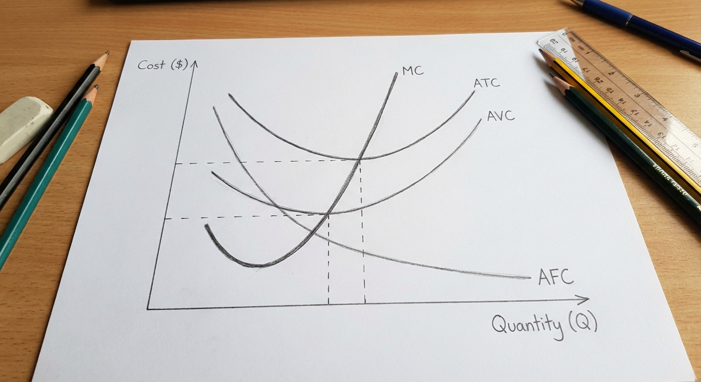
Per-Unit (Average) Costs
- Average Fixed Cost ($AFC$): $\frac{FC}{Q}$ (Always declines as Q increases—"spreading the overhead").
- Average Variable Cost ($AVC$): $\frac{VC}{Q}$ (U-shaped).
- Average Total Cost ($ATC$): $\frac{TC}{Q}$ or $AFC + AVC$ (U-shaped).
- Marginal Cost ($MC$): The cost of producing one additional unit.
Shape and Relationships of Cost Curves
The $MC$ curve looks like a "Nike swoosh." The $ATC$ and $AVC$ curves are U-shaped.
The Most Important Rules for Graphing:
- MC crosses ATC and AVC at their respect minimum points.
- The vertical distance between $ATC$ and $AVC$ represents $AFC$. As quantity increases, this gap gets smaller (because AFC approaches zero).
3.3 Long-Run Production Costs
In the long run, all inputs are variable. A firm can build a bigger factory or sell their equipment. The Long-Run Average Total Cost (LRATC) curve acts as an "envelope" curve that holds all possible short-run ATC curves.
Scale Concepts
- Economies of Scale: As a firm gets bigger (output rises), long-run average costs fall. Caused by specialization, bulk purchasing, and better technology.
- Constant Returns to Scale: Output costs remain constant as the firm grows.
- Diseconomies of Scale: As a firm gets too massive, long-run average costs rise. Caused by management bureaucracy and miscommunication.
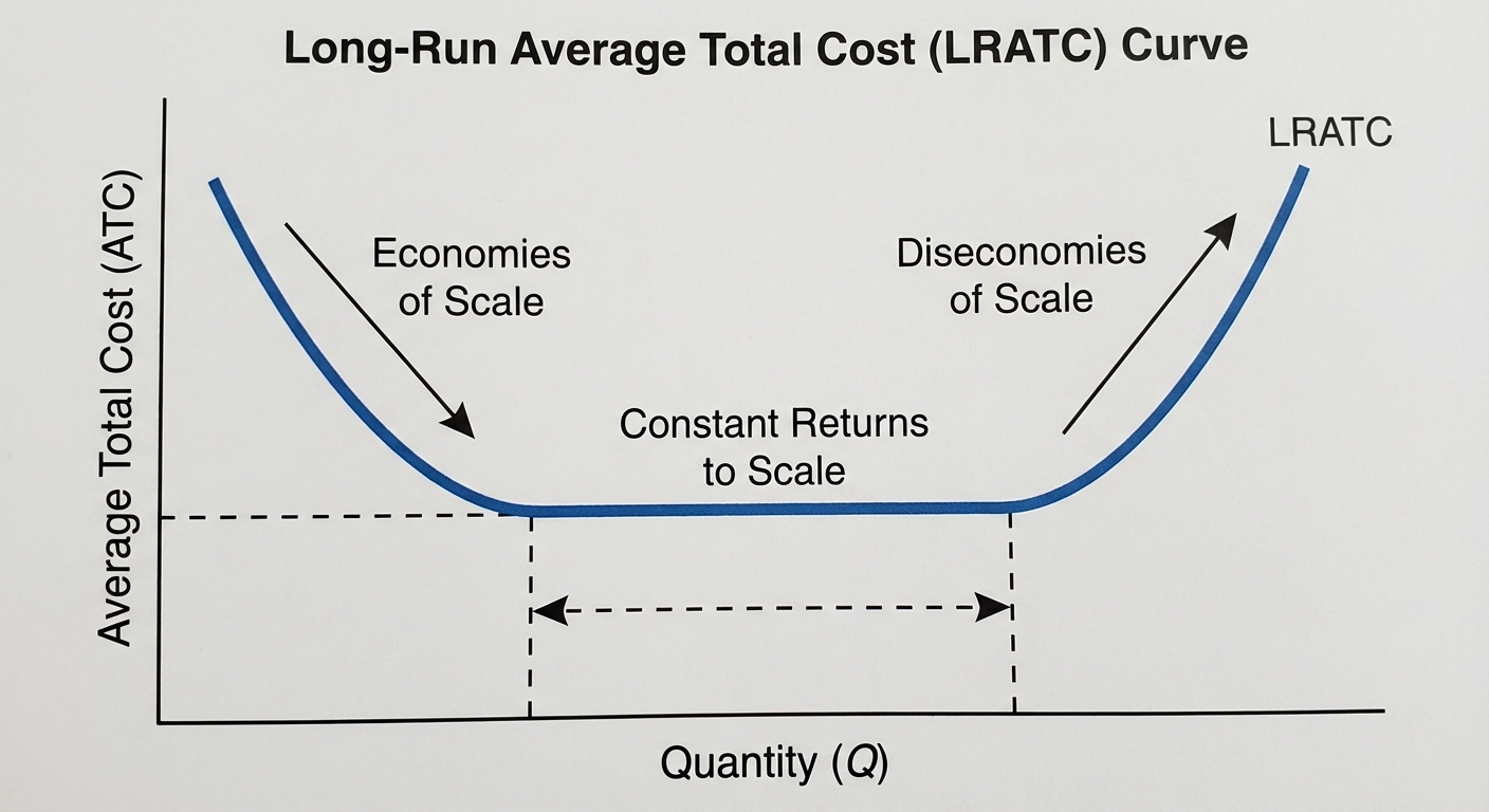
Common Mistakes
- Mistake: Confusing Diminishing Marginal Returns with Diseconomies of Scale.
- Correction: Diminishing Returns happens in the Short Run because of fixed resources. Diseconomies of Scale happens in the Long Run due to management issues.
3.4 Types of Profit
Economists and accountants view "cost" differently.
Explicit vs. Implicit Costs
- Explicit Costs: Out-of-pocket monetary payments (Wages, rent, materials). This is what accountants care about.
- Implicit Costs: The Opportunity Costs of doing business. It is the money you could have earned doing the next best alternative (e.g., the salary the owner gave up to start the business, or the foregone rent on a building the firm owns).
Calculating Profit
- Accounting Profit:
- Economic Profit:
Note: If Economic Profit is Zero, the firm is making a Normal Profit. This means the firm is covering all costs (including the owner's salary) and should stay in business. It is breaking even in an economic sense.
3.5 Profit Maximization
This is the "Golden Rule" of Microeconomics. All firms, regardless of market structure, assume this goal.
The Rule: MR = MC
To maximize profit (or minimize loss), a firm should produce at the quantity where Marginal Revenue equals Marginal Cost.
- If $MR > MC$: produce more (you make profit on the next unit).
- If $MC > MR$: produce less (you are losing money on the last unit).
- The optimal quantity ($Q$) is always found where $MR$ and $MC$ intersect.
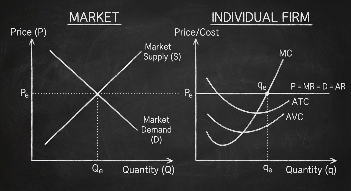
3.6 Perfect Competition: Characteristics
Perfect Competition is a theoretical market structure that serves as a benchmark for efficiency.
Characteristics (Use the mnemonic "PLIGS")
- Price Takers: Firms have no control over price; the market sets it.
- Large number of buyers and sellers.
- Identical Products (Homogeneous goods): Corn, wheat, strawberries.
- Go for ease of Entry/Exit: Low barriers to start or stop the business.
- Side-by-Side Graphs: You must graph the Market and the Firm together.
Demand for the Firm
Because the firm is a price taker, they can sell as much as they want at the market price, but nothing above it. Their demand curve is Perfectly Elastic (Horizontal).
"Mr. DARP" reminds us that for a perfectly competitive firm:
3.7 Short-Run and Long-Run Decisions
Short-Run Production Decisions
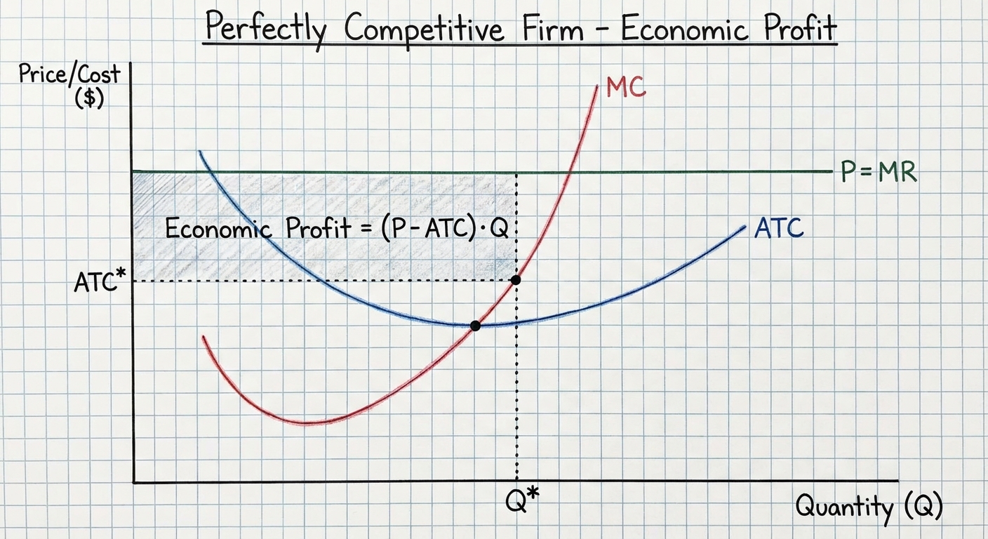
Once a firm finds the profit-maximizing quantity ($MR=MC$), they look at the Average Total Cost ($ATC$) to determine profit.
- Profit ($P > ATC$): The firm is making economic profit.
- Loss ($P < ATC$): The firm is losing money.
- Break-Even ($P = ATC$): The firm is making normal profit (Zero economic profit).
The Shutdown Rule:
If a firm is losing money, should it stop immediately?
- Continue Producing: If $P > AVC$. The price covers the variable costs and contributes some to fixed costs. You lose less by producing than by shutting down.
- Shut Down: If $P < AVC$. The price doesn't even cover the wages/materials. Shut down immediately to limit loss to just Fixed Costs.
Long-Run Adjustment (Entry and Exit)
In the long run, firms can enter or leave the market based on economic profits.
If firms are making PROFIT:
- New firms enter the market.
- Market Supply shifts Right.
- Market Price Falls.
- Firm's $MR$ falls until Profit = 0.
If firms are making a LOSS:
- Firms leave the market.
- Market Supply shifts Left.
- Market Price Rises.
- Firm's $MR$ rises until Profit = 0.
Long-Run Equilibrium:
In the long run, perfectly competitive firms effectively always make Zero Economic Profit. The Price will settle at the minimum of the ATC curve.
Efficiency at Long-Run Equilibrium:
- Productive Efficiency: Producing at lowest cost ($P = \text{minimum } ATC$).
- Allocative Efficiency: Producing what society wants ($P = MC$).
Summary of Formulas
| Concept | Formula |
|---|---|
| Marginal Product ($MP$) | $\Delta TP / \Delta L$ |
| Total Cost ($TC$) | $FC + VC$ |
| Average Total Cost ($ATC$) | $TC / Q$ |
| Marginal Cost ($MC$) | $\Delta TC / \Delta Q$ |
| Profit Maximization | $MR = MC$ |
| Profit | $(P - ATC) \times Q$ |
Common Mistakes & Pitfalls
- Confusing Total Product with Marginal Product: Remember, $MP$ is the slope of $TP$. When $TP$ is maximized, $MP$ is zero.
- Shifting Curves on the Firm Graph: In Perfect Competition, the firm usually does not shift supply. The Market shifts supply, which changes the price, which shifts the firm's $MR$ curve (Mr. DARP).
- Drawing the MC curve wrong: Always ensure $MC$ cuts through the minimum point of both the $AVC$ and $ATC$ curves. If you draw it differently, you will lose points.
- Stopping at MR=MC: Finding where lines cross gives you quantity ($Q$). You must assume a dotted line goes down to the X-axis for $Q$, and up to the Demand curve for Price ($P$). To find cost, go from that $Q$ quantity up/down to the $ATC$ curve.