AP Calculus BC Unit 4: Contextual Applications of Differentiation (Interpretation, Motion, Related Rates, Linearization, and L’Hospital’s Rule)
Interpreting the Derivative in Context
A big shift in Unit 4 is that the derivative stops being “just a procedure” and becomes a meaningful quantity you interpret in words, with units, and in real situations. On the AP Exam, many problems are less about symbolic differentiation and more about explaining what a derivative value tells you about a situation.
The derivative as a rate of change (the core idea)
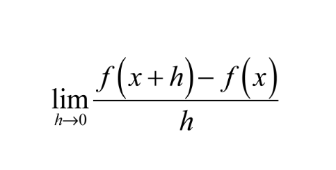
The derivative of a function at an input value measures how fast the output is changing with respect to the input at that instant. Formally, it comes from the limit of average rates of change.
The fraction is an average rate of change over an interval of length , and the limit converts that average into an instantaneous rate. This matters because many real-world quantities are naturally “per unit input” (miles per hour, dollars per item, liters per minute). The derivative is the mathematical tool that captures that “per” relationship at a specific moment.
The derivative as slope (geometry meets context)
If a function is differentiable at a point, its graph has a tangent line there, and the derivative equals the slope of that tangent line.
That connects directly to “rate” language, since slope is “rise over run.”
Units: the fastest way to make your interpretation correct
A derivative always has units of output per input. For example, if an output is measured in meters and the input is measured in seconds, then the derivative has units
This is not optional decoration: units tell you what the derivative means.
- If a population function has units of people and time in years, the derivative has units of people per year.
- If a cost function has units of dollars and input is items produced, the derivative has units of dollars per item (marginal cost).
A common student mistake is to interpret %%LATEX5%% as “the value of the function.” A quick unit-check catches this: %%LATEX6%% has output units, while has output-per-input units.
Sign and magnitude: what does positive, negative, large, or small mean?
Interpreting a derivative is often about sign and size.
- If %%LATEX8%%, then the function is increasing at %%LATEX9%%.
- If %%LATEX10%%, then the function is decreasing at %%LATEX11%%.
- If , the tangent line is horizontal and the quantity is momentarily not changing.
Magnitude matters too.
- A large absolute value means the output is changing rapidly.
- A small absolute value means the output is changing slowly.
Important nuance: does not automatically mean a maximum or minimum in context. It only means “instantaneously flat.” The point could be a local max, a local min, or neither.
Estimating derivatives from graphs, tables, and data
On the AP Exam, you may not be given a formula. You might be given a graph and asked to approximate a tangent slope, or a table and asked to approximate a derivative with a difference quotient.
A strong table-based estimate uses symmetric points around the target input when possible.
If you only have one-sided data, use a one-sided difference quotient.
When you do this, your final answer should include units and an interpretation, not just a number.
Worked example 1: interpreting a derivative value with units
Suppose %%LATEX16%% is the temperature of a cup of coffee in degrees Celsius after %%LATEX17%% minutes, and you are told
This means: at 5 minutes, the coffee’s temperature is decreasing at about 1.8 degrees Celsius per minute. The negative sign indicates cooling.
Worked example 2: estimating a derivative from a table
A table gives the values below. Estimate the derivative at 2.
Use a symmetric difference quotient with .
Interpretation (in general form): at input 2, the function is increasing at about 7.5 output-units per input-unit.
Exam Focus
- Typical question patterns:
- “Interpret in context” given a derivative value.
- “Estimate from a graph/table and explain what it means.”
- “Compare %%LATEX26%% and %%LATEX27%%” to decide where change is faster.
- Common mistakes:
- Giving the meaning of %%LATEX28%% instead of %%LATEX29%% (mixing up value vs. rate).
- Forgetting units or using the wrong units (output vs. output-per-input).
- Treating as automatically “a maximum” without additional justification.
Straight-Line Motion (Position, Velocity, Acceleration)
Motion problems are the most common “derivative in context” problems because everyday language already uses rates: velocity is a rate of change of position, and acceleration is a rate of change of velocity.
The main functions and what they mean
In straight-line motion (movement along a line), you typically have position, velocity, and acceleration connected by derivatives.
A common unit setup is:
- Position measured in meters
- Velocity measured in meters per second
- Acceleration measured in meters per second squared
Here is the same idea organized as a reference table.
| Quantity | Common notation | Typical units |
|---|---|---|
| Position | %%LATEX33%% or %%LATEX34%% | meters |
| Velocity | %%LATEX35%% or %%LATEX36%% | meters per second |
| Acceleration | %%LATEX37%% or %%LATEX38%% or | meters per second squared |
Displacement vs. distance (a crucial conceptual split)
Displacement over a time interval is net change in position.
Distance traveled counts total movement regardless of direction. If velocity exists and is integrable, distance traveled can be found by integrating speed.
Even though Unit 4 emphasizes differentiation, this distinction shows up often as a conceptual trap: speed is absolute value of velocity.
Velocity vs. speed, direction, and “moving right/left”
Velocity can be positive or negative, while speed is always nonnegative.
- If , the object is moving in the positive direction.
- If , the object is moving in the negative direction.
- If , the object is momentarily at rest.
A very common AP phrasing is “moving left,” which is asking for when (assuming the usual coordinate orientation).
When is the object speeding up or slowing down?
Speeding up means the speed is increasing. In straight-line motion, a reliable sign rule is:
- Speeding up when velocity and acceleration have the same sign.
- Slowing down when velocity and acceleration have opposite signs.
This is why “acceleration positive” does not automatically mean “speeding up.” You must compare the signs of both.
Reading motion from graphs
You might be given a graph of position, velocity, or acceleration.
- From a position graph, slope is velocity. Increasing position means positive velocity; decreasing position means negative velocity. Concavity of position relates to acceleration because concavity is controlled by the second derivative.
- From a velocity graph, height is velocity and slope is acceleration. Above the axis means positive direction; below means negative direction; where velocity is zero the object is at rest.
A subtle but important point: a turning point in position (a local max or min) typically happens when velocity is zero and changes sign. But velocity equaling zero alone does not guarantee a direction change.
Worked example 1: interpreting velocity and acceleration from a position function
A particle has position
for nonnegative time.
1) Find velocity and acceleration.
2) When is the particle at rest?
So the particle is at rest at
and
3) Is it speeding up at ?
Because
the sign rule (same sign vs. opposite sign) does not directly decide “speeding up” at that instant. A better approach is to check velocity just before and after.
Velocity changes sign at , so the particle reverses direction there. This highlights the misconception “acceleration positive means speeding up.”
Worked example 2: speeding up intervals
Using the same functions, find where the particle is speeding up.
First find where acceleration is zero.
Velocity factored:
Sign analysis:
- For : velocity positive, acceleration negative, slowing down.
- For : velocity negative, acceleration negative, speeding up.
- For : velocity negative, acceleration positive, slowing down.
- For : velocity positive, acceleration positive, speeding up.
So it is speeding up on
and
Worked example 3: acceleration from a velocity function
If a particle moves along a straight line with velocity
then acceleration is the derivative of velocity.
At time 2,
So at the acceleration is 8 (with units matching your velocity units per second).
Exam Focus
- Typical question patterns:
- Given %%LATEX74%%, find %%LATEX75%% and and interpret at a specific time.
- Determine when the particle moves left/right, is at rest, or changes direction.
- Determine when it is speeding up/slowing down using sign analysis of %%LATEX77%% and %%LATEX78%%.
- Common mistakes:
- Confusing velocity with speed (forgetting the absolute value for speed).
- Saying “speeding up when %%LATEX79%%” instead of checking signs of both %%LATEX80%% and .
- Assuming always means “turns around” without checking sign change.
Rates of Change in Applied Contexts (Other Than Motion)
Once you’re comfortable interpreting derivatives in motion, the same logic applies to any situation where one quantity depends on another: economics, biology, chemistry, geometry, and more. The derivative is still “instantaneous rate of change,” but the meaning changes with the variables.
General interpretation template (a powerful habit)
If an output depends on an input, then the derivative at an input value tells you: when the input equals that value, the output is changing at the derivative amount in output-units per input-unit.
A strong interpretation has three parts:
1) when (at what input),
2) direction (increasing or decreasing),
3) units.
Example statement: if revenue is in dollars and time is in days and
then at day 10 revenue is increasing at 2500 dollars per day.
Average vs. instantaneous rate (and why both appear)
Average rate of change over an interval is
This is not the derivative unless the interval is extremely small. In context, average rate describes the whole interval, while instantaneous rate describes a single moment.
Marginal interpretations (common in economics and modeling)
If cost in dollars depends on number of items produced, then the derivative is marginal cost in dollars per item. It estimates the extra cost of producing one more item near that production level.
For a small change in production,
When
this becomes the “cost of one more item” approximation, which is best when the cost function is smooth.
Chain rule as “rate of a rate” (indirect dependence)
Many real systems are layered: one variable depends on another that depends on time. If a quantity depends on another variable, and that variable depends on time, then the chain rule connects the rates.
Worked example 1: geometric rate of change (area depends on radius)
A circular oil spill has radius and area related by
Suppose
Find the area rate when
Differentiate with respect to time.
Substitute values.
Interpretation: when the radius is 10 meters, the area is increasing at square meters per minute.
Worked example 2: interpreting a rate from a model (biology)
If bacteria population satisfies
then at 3 hours the population is increasing at 500 bacteria per hour. If instead
that does not mean “negative bacteria”; it means the population is decreasing at 500 bacteria per hour at that instant.
Worked example 3: volume changing in a pool (non-motion derivative)
Let volume (in gallons) after time (in hours) be
Then the rate of change of volume is
At
the volume is not changing because
For
the derivative is positive, so the volume is increasing; for
the derivative is negative, so the volume is decreasing.
Worked example 4: coffee cooling model (non-motion derivative)
Suppose coffee temperature (in degrees) is modeled by
where time is minutes since poured. Differentiate to find the rate of change.
At 5 minutes,
So at 5 minutes the temperature is decreasing at about 2.27 degrees per minute.
Exam Focus
- Typical question patterns:
- Interpret %%LATEX105%% or %%LATEX106%% with correct units in a non-motion scenario.
- Use the chain rule with rates (for example, area changing because radius changes).
- Distinguish average rate of change from instantaneous rate of change.
- Common mistakes:
- Dropping units or using the wrong “per” units.
- Forgetting the chain rule factor (for example, missing ).
- Interpreting negative rates as “negative amounts” rather than “decreasing.”
Related Rates: Turning a Situation Into an Equation
A related rates problem is a special kind of rate problem where two or more quantities are connected by a relationship (often geometric). You’re given the rate of change of one quantity and asked to find the rate of change of another.
What makes related rates feel hard at first is not the calculus, but the modeling. The derivative step is usually straightforward. The challenge is translating words into variables and an equation.
What “related” means
The rates are related because the quantities themselves are related. For example, circle area and radius satisfy
If radius changes with time, then area must change with time in a way determined by that equation.
The key move: differentiate with respect to time
Even if the relationship does not explicitly include time, in related rates you treat each changing quantity as a function of time.
For example, if
then differentiating with respect to time gives
This “variable times its time-derivative” pattern is the signature of related rates and comes from the chain rule.
A reliable modeling workflow (what to do before differentiating)
Before you touch derivatives, aim for a clean setup.
- Draw a diagram if geometry is involved. Label variables clearly.
- Choose variables for the quantities that change and include units.
- Write one equation relating the variables.
- Identify the instant: related rates questions always mean “at a particular moment,” and that’s when you plug in numerical values after differentiating.
A common mistake is plugging in numerical values too early. If you substitute before differentiating, you can accidentally erase the variables you need.
Worked example 1: expanding circle (intro-level related rates)
A circle’s radius is increasing at a constant rate of 3 cm/s. Find how fast the area is increasing when the radius is 5 cm.
Given
and
Differentiate with respect to time.
Substitute
and
So at that instant, area is increasing at square centimeters per second.
Worked example 2: a non-obvious given value (finding missing info)
A point moves along
At an instant,
and
Find .
Differentiate with respect to time.
Solve for the desired rate.
Now find the corresponding value using the original equation.
So
or
If the context doesn’t specify which semicircle, both are possible.
If
then
If
then
This is an important modeling point: geometry can create multiple physical positions unless the context restricts a sign.
Worked example 3: area expanding given, solve for radius rate
A pool (circle) is expanding at
square inches per second. Find the rate the radius is expanding when
inches.
Start with
Differentiate with respect to time.
Substitute.
So the radius is increasing at 2 inches per second.
Worked example 4: spherical balloon (volume rate to radius rate)
A spherical balloon is being inflated at
cubic inches per second. How fast is the radius increasing when
inches?
Use the sphere volume formula.
Differentiate with respect to time.
Substitute.
So the radius is increasing at
inches per second.
Exam Focus
- Typical question patterns:
- “Given %%LATEX147%%, find %%LATEX148%%” using an equation like a circle, ellipse, or triangle.
- “At the instant when …” with numerical substitutions after differentiating.
- Situations requiring you to compute an un-given variable value (like finding from a circle equation).
- Common mistakes:
- Substituting numbers before differentiating (which can remove needed variables).
- Forgetting chain rule factors like after differentiating powers.
- Ignoring multiple possible values (for example, ) when the context doesn’t fix a sign.
- Forgetting to include units in the final answer or not checking whether the sign makes sense physically.
Solving Related Rates Problems (Full Strategy + Classic Setups)
Most AP related rates problems follow a predictable structure. Once you develop a method, they become much less mysterious.
A step-by-step strategy you can reuse
Here’s a combined workflow that captures the standard process.
- Read the problem carefully and identify all given information.
- Sketch and label the situation, and note what is constant versus changing.
- Assign variables (not numbers) to the changing quantities, including units.
- Write one relationship equation connecting the variables.
- Differentiate both sides with respect to time.
- Substitute known values for variables and rates at the specified instant.
- Solve for the requested rate and state units.
A helpful memory aid is “ERDS”: Equation, Differentiate, Replace (substitute), Solve.
Classic setup 1: ladder sliding down a wall
A ladder of fixed length makes a right triangle with the wall and floor.
Let
be the distance of the bottom from the wall and
be the height of the top on the wall. If ladder length is constant , then
Differentiate with respect to time.
Solve for the top’s vertical rate.
The sign is meaningful: if %%LATEX158%% (bottom moving away), then %%LATEX159%% (top moving down).
Worked ladder example
A 13 ft ladder rests against a wall. The bottom slides away at 2 ft/s. How fast is the top sliding down when the bottom is 5 ft from the wall?
Given
and evaluate at
First find .
Now compute.
So the top is sliding down at ft/s (negative indicates downward if up is positive).
Common pitfall: mixing up which distance is %%LATEX169%% and which is %%LATEX170%%, then interpreting the sign incorrectly.
Classic setup 2: related rates with volume (cones, spheres, cylinders)
These problems often give a filling or draining rate such as and ask for a height or radius rate. The key modeling move is often rewriting volume in terms of one variable using similar triangles.
Worked cone example (with similar triangles)
Water is poured into an inverted right circular cone at a constant rate of
ft/min. The cone has height 10 ft and radius 4 ft. How fast is the water level rising when the water is 5 ft deep?
Start with the cone volume.
Use similar triangles to relate radius and height. The full cone ratio is
So for the water surface,
Substitute into volume so volume depends only on .
Differentiate with respect to time.
Substitute
and
So the water level is rising at ft/min when the depth is 5 ft.
Common pitfalls:
- Forgetting to relate %%LATEX186%% and %%LATEX187%% using similar triangles.
- Differentiating with respect to %%LATEX188%% instead of %%LATEX189%%.
- Plugging too early before differentiation is complete.
Classic setup 3: shadows and similar triangles
Shadow problems follow a consistent pattern: use similar triangles to relate heights and shadow lengths, then differentiate with respect to time. A frequent mistake is flipping ratios or mixing which triangle corresponds to which measurement.
Exam Focus
- Typical question patterns:
- Ladder or moving-point problems using Pythagorean theorem with implicit differentiation.
- Volume problems requiring similar triangles to eliminate a variable before differentiating.
- Word problems that hide which quantities are changing versus constant.
- Common mistakes:
- Using the wrong geometric relationship (for example, using full cone dimensions directly in volume without similar triangles).
- Treating constants as variables or variables as constants (especially ladder length).
- Dropping negative signs that communicate direction (downward vs. upward, shrinking vs. growing).
- Not including units or not checking whether the result is physically reasonable.
Local Linearization and Differentials (Approximating Function Values)
Not every real situation needs an exact value. Sometimes you need a fast, accurate approximation. Local linearization uses the derivative to approximate a function near a point where you already know the function value.
The big idea: a function looks linear close to a point
If a function is differentiable at a point, then near that point the graph is well-approximated by its tangent line.
The tangent-line approximation (linearization) at is
For %%LATEX193%% close to %%LATEX194%%,
Connecting linearization to “small change” formulas
Some notes describe a “small change” using %%LATEX196%% (a small input change), while calculus differentials often use %%LATEX197%%. The key idea is the same: small input changes produce approximately linear output changes.
Differentials are packaged as
Near , you often compute
Another common linearization form (equivalent to the tangent line idea) is
This can be motivated by the limit definition: it’s like “replace %%LATEX202%% with %%LATEX203%% and remove the limit,” turning the exact derivative relationship into an approximation for small changes.
How to choose the point
Pick %%LATEX204%% so that %%LATEX205%% is easy to compute and your target value is close to . For approximating a square root, choose a nearby perfect square.
Worked example 1: approximating a square root
Approximate using linearization.
Let
Choose
Then
Derivative:
So
Linearization:
Evaluate at 50.
So
Common mistake: choosing a convenient point that is not close (for example, using %%LATEX216%% for %%LATEX217%%), which reduces accuracy.
Worked example 2: using differentials to estimate measurement error
A sphere has volume
Suppose
cm with possible measurement error
cm. Estimate the resulting error in volume.
Differentiate with respect to .
Use differentials.
Substitute.
So the volume error is about %%LATEX225%% cm%%LATEX226%%.
Worked example 3: differential approximation of a power
Use a differential (linear approximation) to approximate
Let
Choose a nearby convenient value
and a small change
Compute
and
so
Use the approximation
Then
You can check this on a calculator to see the approximation is very close.
When linearization can mislead (and how concavity helps)
Linearization is local: it works best when the target input is close to the base point and the function isn’t curving too sharply near that point. If concavity is known, you can often justify whether the tangent-line approximation is an overestimate or underestimate: concave up functions lie above tangent lines, and concave down functions lie below.
Exam Focus
- Typical question patterns:
- “Use linearization at %%LATEX236%% to approximate %%LATEX237%% for %%LATEX238%% near %%LATEX239%%.”
- “Find the linearization %%LATEX240%% of %%LATEX241%% at .”
- “Use differentials to estimate change/error” (propagation of measurement error).
- Common mistakes:
- Using a point that is not close to the target value, causing poor approximation.
- Forgetting the structure and instead writing a generic line.
- Confusing %%LATEX245%% (actual change) with %%LATEX246%% (approximate change) and treating them as exactly equal.
- Treating as “the derivative” instead of as a small input change used for approximation.
L’Hospital’s Rule (Limits via Derivatives)
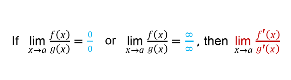
Some AP Calculus problems connect derivatives to evaluating limits. If a limit produces an indeterminate form, L’Hospital’s Rule allows you to differentiate the numerator and denominator and try the limit again.
When you can use it
If a limit results in either indeterminate form below, L’Hospital’s Rule may apply (assuming the functions are differentiable near the point and the limit conditions are met).
- Indeterminate form
- Indeterminate form
What the rule does
If
is of the form %%LATEX251%% or %%LATEX252%%, then you can compute
and see whether that new limit is determinate.
Worked example: repeated application
Evaluate
As %%LATEX255%%, both numerator and denominator grow without bound, so it is an %%LATEX256%% indeterminate form.
Differentiate numerator and denominator once.
This is still , so differentiate again.
Still , differentiate again.
So the limit is
Exam Focus
- Typical question patterns:
- Limits that simplify to %%LATEX263%% or %%LATEX264%%, especially rational functions, exponentials, logs, and trig expressions.
- “Apply L’Hospital’s Rule once” versus cases that require repeated applications.
- Common mistakes:
- Using L’Hospital’s Rule when the form is not %%LATEX265%% or %%LATEX266%%.
- Differentiating incorrectly (especially product/quotient/chain rule errors).
- Forgetting that after each differentiation, you must re-check the limit form before deciding to stop.