Unit 7: Mastery of Differential Equations

Separation of Variables: General and Particular Solutions

Separation of Variables is the primary algebraic technique used in AP Calculus to solve first-order differential equations. The goal is to rewrite the equation so that all terms involving the dependent variable (usually $y$) are on one side with $dy$, and all terms involving the independent variable (usually $x$ or $t$) are on the other side with $dx$.

The Core Concept

Given a differential equation in the form:
\frac{dy}{dx} = g(x)h(y)

You must manipulate the algebra to achieve:
\int \frac{1}{h(y)} \, dy = \int g(x) \, dx

General vs. Particular Solutions

1. General Solution: A family of functions containing an arbitrary constant of integration ($+C$). This represents all possible curves that satisfy the differential rate of change.
2. Particular Solution: A specific function where the constant $C$ has been solved for using an Initial Condition ($y(x0) = y0$). Geometrically, this is the single curve passing through a specific point.

Step-by-Step Procedure

1. Separate: Move variables to opposite sides. Treat $dy$ and $dx$ as separable differentials.
2. Integrate: Perform antiderivatives on both sides independently.
3. Add Constant: Add $+C$ to the side with the independent variable immediately after integrating.
4. Use Initial Condition (if provided): Substitute $(x, y)$ values to solve for $C$.
5. Isolate: Solve for $y$ explicitly if possible.

Worked Example: Particular Solution

Problem: Find the particular solution $y = f(x)$ to the differential equation $\frac{dy}{dx} = xy^2$ with the initial condition $f(0) = -1$.

Solution:

1. Separate: Divide by $y^2$ and multiply by $dx$:
   \frac{1}{y^2} \, dy = x \, dx \implies \int y^{-2} \, dy = \int x \, dx

2. Integrate:
   -y^{-1} = \frac{1}{2}x^2 + C
   -\frac{1}{y} = \frac{1}{2}x^2 + C

3. Apply Initial Condition ($x=0, y=-1$):
   -\frac{1}{-1} = \frac{1}{2}(0)^2 + C \implies 1 = 0 + C \implies C = 1

4. Substitute and Isolate $y$:
   -\frac{1}{y} = \frac{1}{2}x^2 + 1
   y = \frac{-1}{\frac{1}{2}x^2 + 1} = \frac{-2}{x^2 + 2}

Exponential Models with Differential Equations

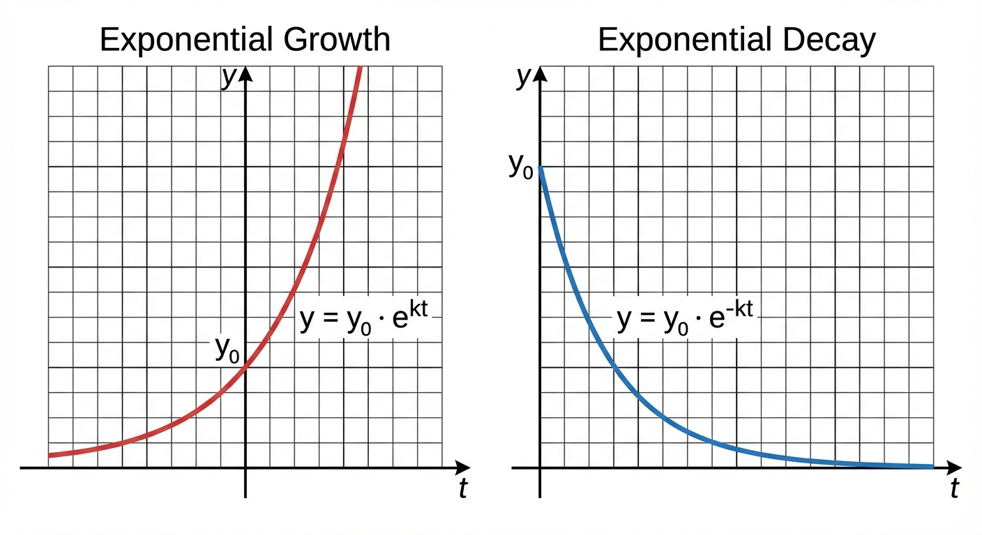
Exponential models describe situations where the rate of change of a quantity is directly proportional to the quantity itself. This is common in population genetics, radioactive decay, and continuously compounded interest.

The Differential Equation

The standard form for exponential growth or decay is:

\frac{dy}{dt} = ky

• $y(t)$: The quantity at time $t$
• $k$: The constant of proportionality
  • If $k > 0$: Exponential Growth
  • If $k < 0$: Exponential Decay

The General Solution

Solving this via separation of variables yields a result you should memorize for efficiency:

\int \frac{1}{y} \, dy = \int k \, dt \implies \ln|y| = kt + C \implies |y| = e^{kt+C} \implies y = Ae^{kt}

Where $A = e^C$ represents the initial value $y_0$ (at $t=0$).

Final Formula:
y(t) = y_0 e^{kt}

Worked Example: Radioactive Decay

A substance decays at a rate proportional to its mass. Half of the substance remains after 10 years. If the initial mass is 100g, find the mass formula.

1. Model: $y(t) = y0 e^{kt}$. We know $y0 = 100$.
2. Use Half-Life: At $t=10$, $y = 50$.
   50 = 100 e^{k(10)}
   0.5 = e^{10k}
   \ln(0.5) = 10k \implies k = \frac{\ln(0.5)}{10} \approx -0.0693
3. Solution: $y(t) = 100 e^{-0.0693t}$

Logistic Models with Differential Equations

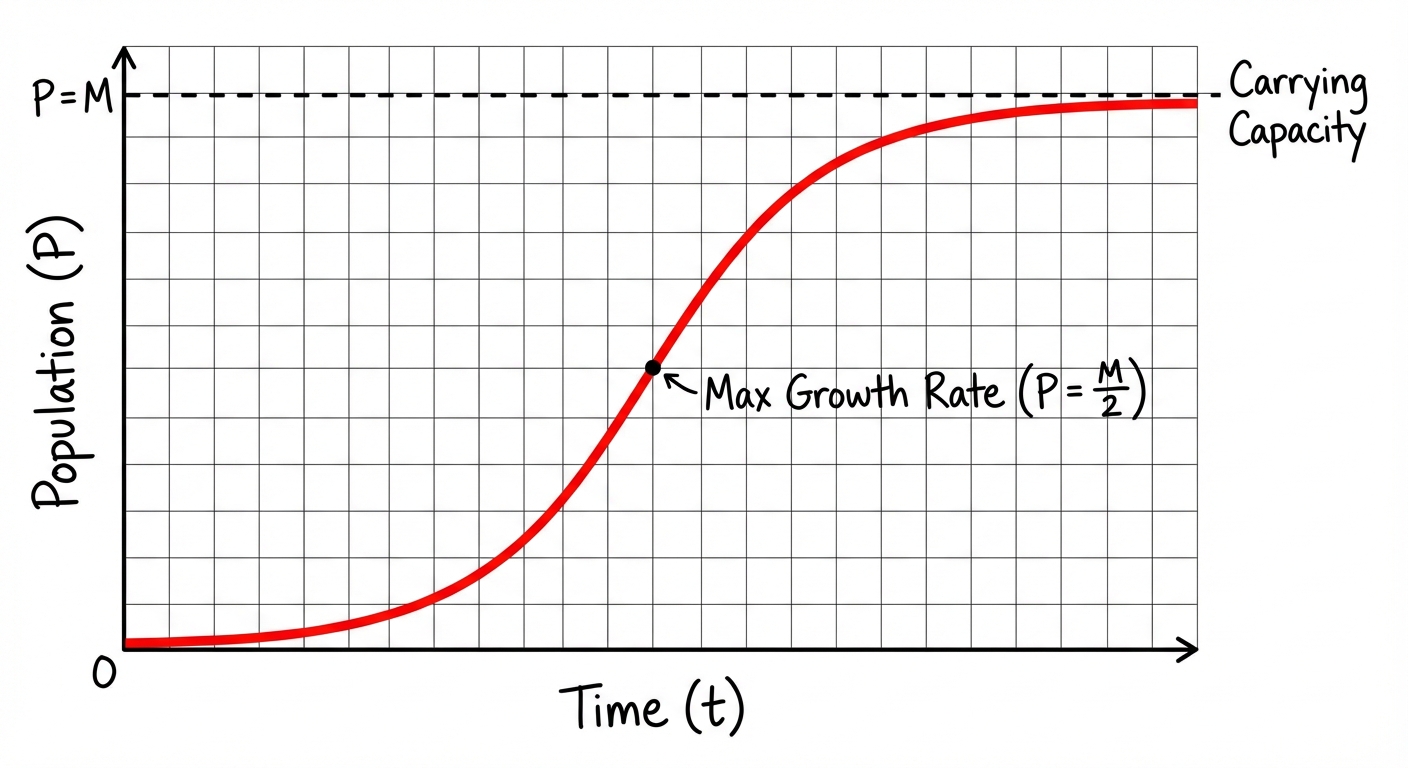
While exponential growth assumes unlimited resources, Logistic Growth models real-world population dynamics where growth is limited by density-dependent factors (e.g., food, space). This limit is called the Carrying Capacity ($M$ or $L$).

The Differential Equation

There are two common forms of the logistic differential equation used on the AP exam:

1. Factorized form:
   \frac{dP}{dt} = kP \left(1 - \frac{P}{M}\right)

   • $k$: Maximum relative growth rate
   • $M$: Carrying capacity

2. Expanded form (using a different constant $c$):
   \frac{dP}{dt} = cP(M - P)

   • Note: Here, the constant $c = \frac{k}{M}$.

Key Features of Logistic Growth

Understanding the behavior of the differential equation is often tested more heavily than solving it completely.

• Limits:
  \lim_{t \to \infty} P(t) = M
  The population always approaches the carrying capacity.
• Growth Rates:
  • If $P < M$: $\frac{dP}{dt} > 0$ (Population grows)
  • If $P > M$: $\frac{dP}{dt} < 0$ (Population shrinks)
• Maximum Growth Rate:
  The population grows fastest (steepest tangent line/inflection point) exactly when the population is half the carrying capacity:
  P = \frac{M}{2}

Solving the Logistic Equation

To solve $\frac{dP}{dt} = kP(1 - \frac{P}{M})$, you must use Partial Fraction Decomposition.

1. Separate: $\int \frac{1}{P(M-P)} \, dP = \int \frac{k}{M} \, dt$
2. Decompose: $\frac{1}{P(M-P)} = \frac{1/M}{P} + \frac{1/M}{M-P}$
3. The general solution is usually given as:
   P(t) = \frac{M}{1 + Ae^{-kt}}
   (where $A$ is a constant determined by the initial population)

Common Mistakes & Pitfalls

1. The "Placement of C" Error

Mistake: Adding $+C$ at the very end of the problem after doing algebra on $y$.
Correction: You must add $+C$ immediately after integrating the $x$-side. For example, if you integrate to get $\ln|y| = x^2$, writing $y = e^{x^2} + C$ is WRONG. It must be $\ln|y| = x^2 + C \to y = e^{x^2+C} \to y = Ae^{x^2}$.

2. Forgetting Absolute Values

Mistake: Writing $\int \frac{1}{y} dy = \ln(y)$.
Correction: The integral is $\ln|y|$. While the absolute value often disappears due to initial conditions being positive (like population or mass), you must start with it to verify the domain.

3. Logistic Carrying Capacity Confusion

Mistake: Identifying the carrying capacity incorrectly from the equation $\frac{dP}{dt} = 0.2P(100 - P)$.
Correction: The standard form is $kP(1 - \frac{P}{M})$. If the equation is $c P(M - P)$, $M$ is the number inside the parenthesis. In $0.2P(100-P)$, the carrying capacity is $100$. However, if written as $0.2P(1 - \frac{P}{100})$, the capacity is also $100$. Watch algebraic forms closely.