AP Microeconomics Unit 6: Market Failure and the Role of Government
6.1 Socially Efficient and Inefficient Market Outcomes
Defining Efficiency and Market Failure
In previous units, we assumed markets were perfectly competitive and functioning without interference. In Unit 6, we analyze what happens when markets fail to allocate resources efficiently.
Market Failure occurs when the free market system fails to allocate resources efficiently, meaning the market equilibrium quantity does not equal the socially optimal quantity ($Q{market} \neq Q{optimal}$).
To understand this, we must distinguish between private and social costs/benefits:
- Marginal Private Cost (MPC): The cost for the firm to produce one more unit (Supply Curve).
- Marginal Private Benefit (MPB): The benefit to the consumer of consuming one more unit (Demand Curve).
- Marginal Social Cost (MSC): The total cost to society (Private Cost + External Cost).
- Marginal Social Benefit (MSB): The total benefit to society (Private Benefit + External Benefit).
The Golden Rule of Allocative Efficiency
A market is Allocatively Efficient (Socially Optimal) only when:
In a perfectly competitive market with no externalities, $MPC = MSC$ and $MPB = MSB$, so the market equilibrium ($Supply = Demand$) is socially efficient. When externalities exist, this equality breaks.
6.2 Externalities
An Externality is a cost or benefit imposed on a third party who is not involved in the transaction (neither the buyer nor the seller). These cause the market to fail because the decision-makers do not consider the full social impact of their actions.
Negative Externalities (Spillover Costs)
Occurs when the social cost is greater than the private cost ($MSC > MPC$). The free market overallocates resources to this good.
- Example: Pollution/Smoking. A factory produces steel (private cost) but pollutes the air (external cost).
- Result: The market produces too much ($Q{mkt} > Q{soc}$) at too low a price.
- Deadweight Loss (DWL): Exists because units are produced where $MSC > MSB$.
- Visual: The MSC curve is above (to the left of) the MPC curve. The vertical distance between them is the Marginal External Cost.

Government Solution: Per-Unit Tax. This shifts the MPC curve to the left (up), aligning it with the MSC curve, forcing the firm to internalize the externality.
Positive Externalities (Spillover Benefits)
Occurs when the social benefit is greater than the private benefit ($MSB > MPB$). The free market underallocates resources to this good.
- Example: Education/Vaccines. You pay for a vaccine (private benefit), but society gains because you won't spread disease (external benefit).
- Result: The market produces too little ($Q{mkt} < Q{soc}$) at too low a price.
- Visual: The MSB curve is above (to the right of) the MPB curve. The vertical distance is the Marginal External Benefit.
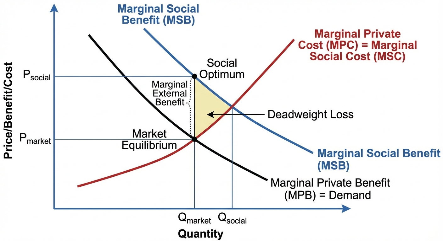
Government Solution: Per-Unit Subsidy. This shifts the MPB curve right (or MPC curve right), encouraging consumption/production to the socially optimal level.
Comparison Table
| Type | Inequality | Market Output vs Social Output | Policy Solution |
|---|---|---|---|
| Negative Externality | $MSC > MPC$ | Overproduced ($Qm > Qs$) | Per-Unit Tax |
| Positive Externality | $MSB > MPB$ | Underproduced ($Qm < Qs$) | Per-Unit Subsidy |
The Coase Theorem
If property rights are clearly defined and transaction costs are low/zero, private parties can bargain to solve the externality problem without government intervention.
6.3 Public and Private Goods
Goods are classified based on two criteria:
- Rivalry: Does one person's consumption prevent another from consuming it?
- Excludability: Can people be prevented from using the good if they don't pay?

1. Private Goods
- Rival & Excludable.
- Examples: Pizza, shoes, cars.
- these are efficiently provided by private markets.
2. Public Goods
- Non-Rival & Non-Excludable.
- Examples: National defense, street lights, lighthouse, clean air.
- Market Failure: Private markets underproduce or do not produce these at all.
- The Free-Rider Problem: Because the good is non-excludable, individuals have no incentive to pay for it, hoping others will pay while they still benefit. The government must provide these goods using tax revenue.
3. Club Goods (Artificially Scarce)
- Non-Rival & Excludable.
- Examples: Cable TV, subscription software, private parks.
- Usually provided by natural monopolies.
4. Common Resources
- Rival & Non-Excludable.
- Examples: Fish in the open ocean, clean water in a river.
- Tragedy of the Commons: Because no one owns the resource (non-excludable) but consumption depletes it (rival), individuals act in self-interest and deplete the resource (over-consumption/over-fishing).
6.4 Government Intervention
When markets fail, governments intervene using taxes, subsidies, price controls, or regulation. The impact of these interventions (tax incidence) depends on elasticity.
Types of Intervention
1. Per-Unit vs. Lump-Sum (Crucial for AP)
- Per-Unit Tax/Subsidy: Affects Marginal Cost (MC), AVC, and ATC. Because MC changes, the profit-maximizing quantity ($MR=MC$) changes.
- Effect: Changes Output ($Q$) and Price ($P$).
- Lump-Sum Tax/Subsidy: A one-time fixed cost/benefit. Affects Fixed Costs (FC) and ATC, but NOT Marginal Cost.
- Effect: Changes Profit, but does NOT change Output ($Q$) or Price ($P$) in the short run.
2. Price Controls (Review)
- Price Ceiling: Max price below equilibrium. Causes Shortage.
- Price Floor: Min price above equilibrium. Causes Surplus.
3. Antitrust Policy
Government laws designed to promote competition and limit monopoly power.
- Sherman Antitrust Act: Outlaws "conspiracy in restraint of trade" (collusion) and monopolization.
- Goal: Increase quantity produced and lower prices to closer align with the allocative efficiency point ($P=MC$).
6.5 Inequality and Income Distribution
Markets reward productivity, not equality. This leads to uneven income distribution.
Measuring Inequality: The Lorenz Curve
The Lorenz curve graphically represents the distribution of income.
- X-axis: Cumulative % of Population.
- Y-axis: Cumulative % of Income.
- Line of Perfect Equality: A 45-degree straight line where 20% of the population has 20% of income, 50% has 50%, etc.

The Gini Coefficient
A mathematical ratio representing the degree of inequality.
- Area A: The gap between the Line of Perfect Equality and the Lorenz Curve.
- Area B: The area under the Lorenz Curve.
- Range: $0$ to $1$.
- $0$ = Perfect Equality (Everyone has same income).
- $1$ = Perfect Inequality (One person has all the income).
Sources of Income Inequality
- Abilities/Human Capital: Differences in education, skills, and experience.
- Discrimination: In hiring or wages.
- Inheritance: Accumulated wealth passed down.
- Market Power: Strong unions or monopolies influencing wages.
Tax Structures
Policies to address inequality rely on different tax systems:
- Progressive Tax: Higher income earners pay a higher percentage of their income.
- Effect: Reduces inequality.
- Example: US Federal Income Tax.
- Proportional (Flat) Tax: Everyone pays the same percentage regardless of income.
- Effect: No change in relative inequality.
- Regressive Tax: Higher income earners pay a lower percentage of their income (often simply a flat dollar amount creates this effect).
- Effect: Increases inequality.
- Example: Sales tax (takes a larger % of a poor person's income than a rich person's).
Common Mistakes & Pitfalls
- Lump-Sum vs. Per-Unit: Students frequently forget that a Lump-Sum tax/subsidy does NOT change the quantity produced ($Q$) because it does not shift the MC curve. If the problem implies a fixed cost change, leave $Q$ alone!
- Naming the Curves: In Unit 6, stop using just "Supply" and "Demand". You must label them MSC/MPC and MSB/MPB to get full credit on Free Response Questions (FRQs).
- Deadweight Loss Arrow: The DWL triangle always points toward the socially optimal point (where $MSC = MSB$).
- Public Goods: Do not confuse "Public Goods" with "Government funded goods". A public good must be non-rival and non-excludable. Schools are government-funded, but they are rival (classrooms fill up) and excludable (you can be suspended), so they are not pure public goods.
- Externalities Calculation: Remember that $MSC = MPC + Marginal External Cost$. If the external cost is constant, the distance between the supply curves is constant.