Comprehensive Guide to Parametrics, Vectors, and Matrices
4.1 Parametric Functions
Definitions & Concepts
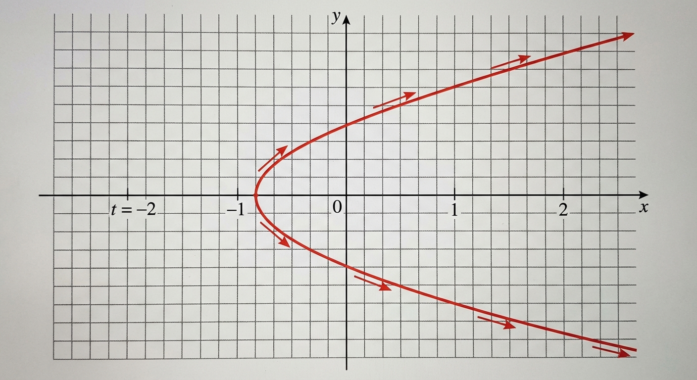
Parametric functions allow us to define curves that are not necessarily functions of $x$ (i.e., they can fail the vertical line test). Instead of relating $y$ directly to $x$, we define both variables in terms of a third independent variable called the parameter, usually denoted by $t$.
- Notation: A parametric function is written as a set of equations: $x = f(t)$ and $y = g(t)$.
- Coordinate Points: At any specific value $t$, the coordinate is $(f(t), g(t))$.
- Orientation: The direction the graph is traced as $t$ increases is called the orientation of the curve.
Graphing Parametric Functions
To graph a parametric equation:
- Create a table with columns for $t$, $x(t)$, and $y(t)$.
- Select values for $t$ within the given domain.
- Calculate the resulting $(x, y)$ coordinate pairs.
- Plot points and connect them in order of increasing $t$.
Eliminating the Parameter
To convert a parametric equation to a Cartesian (rectangular) equation ($y=f(x)$):
- Solve one equation for $t$ (e.g., $t = x/2$).
- Substitute this expression into the other equation.
Example:
Given $x = 2t$ and $y = t^2 + 1$:
- Solve for $t$: $t = \frac{x}{2}$.
- Substitute into $y$: $y = (\frac{x}{2})^2 + 1 \Rightarrow y = \frac{x^2}{4} + 1$.
4.2 Parametric Functions Modeling Planar Motion
Analyzing Particle Motion
In physics and applied mathematics, parametric equations often model the position of a particle at time $t$.
- $x(t)$: The horizontal position of the particle.
- $y(t)$: The vertical position of the particle.
- Domain: Usually $t \geq 0$ (time cannot be negative), but context determines the domain.
Extrema (Maximums and Minimums)
To find the boundaries of motion:
- Horizontal Extrema: Find the maximum and minimum values of $x(t)$. These represent the usually "rightmost" and "leftmost" points.
- Vertical Extrema: Find the maximum and minimum values of $y(t)$. These represent the "highest" and "lowest" points.
Example:
If $x(t) = \sin(t)$ and $y(t) = t^2$ on $[0, \pi]$:
- Max horizontal Position: $x=1$ at $t=\pi/2$.
- Max vertical Position: $y=\pi^2$ at $t=\pi$.
4.3 Parametric Functions and Rates of Change
Direction of Motion
To understand how a particle moves, we analyze the rate of change of $x$ and $y$ independently.
| Condition | Interpretation |
|---|---|
| $x$ is increasing | Particle moves to the right |
| $x$ is decreasing | Particle moves to the left |
| $y$ is increasing | Particle moves up |
| $y$ is decreasing | Particle moves down |
Average Rate of Change (AROC)
The average rate of change describes how the position changes over an interval $[a, b]$. Unlike standard functions, we calculate AROC for each component separately:
- AROC of x: $\frac{x(b) - x(a)}{b - a}$ (Average horizontal velocity)
- AROC of y: $\frac{y(b) - y(a)}{b - a}$ (Average vertical velocity)
4.4 Parametrically Defined Functions
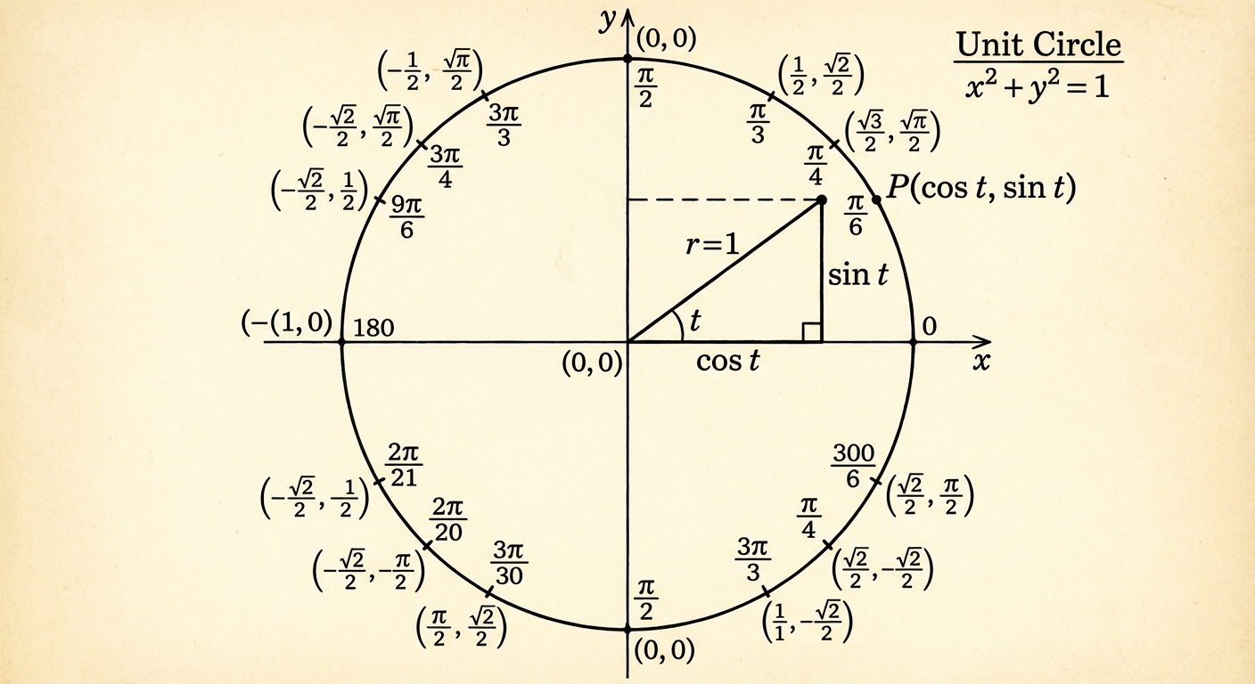
Parametrizing Circles
The Unit Circle is the foundation for parametrizing circular motion. Based on the Pythagorean identity $\cos^2 \theta + \sin^2 \theta = 1$:
General Standard Form for a Circle:
- $(xc, yc)$: Center of the circle.
- $r$: Radius.
- $t$: Angle parameter (often $\theta$).
- Period: Standard circle completes in $2\pi$. If the argument is $bt$, the period changes to $2\pi/b$.
Parametrizing Line Segments
To describe linear motion from Point A $(x1, y1)$ to Point B $(x2, y2)$:
- For $0 \leq t \leq 1$, the particle starts at A and ends at B.
4.5 Implicitly Defined Functions
Concepts
An implicitly defined function relates $x$ and $y$ in a single equation where one variable is not isolated (e.g., $x^2 + y^2 = 25$ or $x^3 + y^3 = 9xy$).
- Verifying Points: To check if a point $(a, b)$ is on the graph, substitute $x=a$ and $y=b$. If the equation yields a true statement (e.g., $25=25$), the point lies on the curve.
- Graphing: These often define non-functions (like circles, ellipses, or hyperbolas) which may require solving for $y$ (often resulting in $\pm$ square roots) to graph on a standard calculator.
4.6 Conic Sections
We can represent conic sections using parametric equations to easily graph and analyze them.
Ellipses
For an ellipse centered at $(h, k)$ with horizontal radius $a$ and vertical radius $b$:
- Implicit: $\frac{(x-h)^2}{a^2} + \frac{(y-k)^2}{b^2} = 1$
- Parametric:
for $0 \leq t \leq 2\pi$.
Hyperbolas
For a hyperbola opening horizontally:
- Implicit: $\frac{(x-h)^2}{a^2} - \frac{(y-k)^2}{b^2} = 1$
- Parametric:
4.8 Vectors
Vector Fundamentals
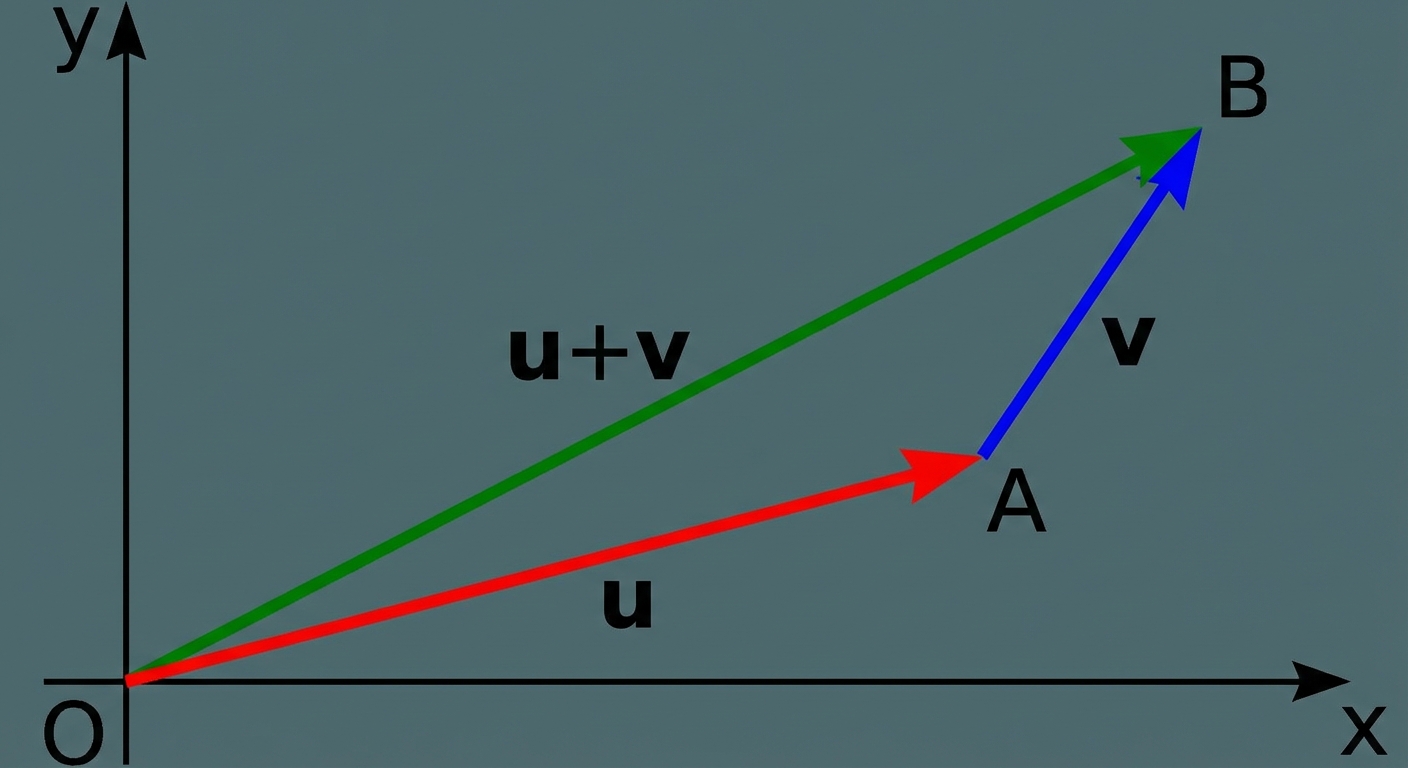
A Vector is a quantity defined by both magnitude (length) and direction. It is represented geometrically as a directed line segment (arrow).
- Component Form: $\mathbf{v} = \langle a, b \rangle$. This represents the change in $x$ ($a$) and the change in $y$ ($b$) from the tail to the head.
- Zero Vector: $\mathbf{0} = \langle 0, 0 \rangle$.
Magnitude and Direction
Given vector $\mathbf{v} = \langle a, b \rangle$:
- Magnitude ($||\mathbf{v}||$): Pythagorean theorem.
- Direction Angle ($\theta$): Using trigonometry.
Note: You must adjust $\theta$ based on the quadrant where $(a,b)$ is located.
Vector Operations
Given $\mathbf{u} = \langle u1, u2 \rangle$, $\mathbf{v} = \langle v1, v2 \rangle$, and scalar $k$:
- Addition: $\mathbf{u} + \mathbf{v} = \langle u1+v1, u2+v2 \rangle$
- Scalar Multiplication: $k\mathbf{u} = \langle k u1, k u2 \rangle$
4.9 Vector-Valued Functions
Position Vectors
A vector-valued function $\mathbf{p}(t)$ describes the position of a particle at time $t$ as a vector from the origin $(0,0)$ to the point $(x(t), y(t))$.
- Radius: The magnitude $||\mathbf{p}(t)||$ represents the distance of the particle from the origin.
Velocity Vectors
The velocity vector $\mathbf{v}(t)$ represents the instantaneous speed and direction of motion.
- If position is linear, velocity is constant.
- Speed: The magnitude of the velocity vector is the speed of the particle.
4.10 Matrices
Concepts & Notation
A Matrix is a rectangular array of numbers. Dimensions are given as $Rows \times Columns$ ($R \times C$).
- This is a $2 \times 3$ matrix (2 rows, 3 columns).
- Element $a_{2,3}$ is the entry in Row 2, Column 3 (value is 6).
Matrix Multiplication
To multiply Matrix $A$ ($m \times n$) by Matrix $B$ ($n \times p$), the inner dimensions ($n$) must match. The result will be size $m \times p$.
The Rule: Row by Column
To find the entry in, say, row 1 column 1 for the result, you take the Dot Product of Row 1 from Matrix A and Column 1 from Matrix B.
Mnemonics:
RC Cola: Always multiply Rows by Columns.
4.11 The Inverse and Determinant of a Matrix
The Determinant
For a $2 \times 2$ square matrix $A = \begin{bmatrix} a & b \ c & d \end{bmatrix}$:
- Geometric Meaning: The absolute value $|\det(A)|$ is the area of the parallelogram formed by the vectors $\langle a, c \rangle$ and $\langle b, d \rangle$.
- If $\det(A) = 0$, the matrix is singular (non-invertible).
The Inverse Matrix
The inverse $A^{-1}$ "undoes" matrix A. When multiplied, $A \cdot A^{-1} = I$ (Identity Matrix).
- Note: We swap the main diagonal elements ($a$ and $d$) and negate the other diagonal ($b$ and $c$).
4.12 Linear Transformations and Matrices
Defining Linear Transformations
A transformation $L$ is linear if it preserves vector addition and scalar multiplication. Essentially, it keeps grid lines parallel and the origin fixed.
Any linear transformation from $\mathbb{R}^2$ to $\mathbb{R}^2$ can be defined by a $2 \times 2$ matrix $M$.
Mapping Basis Vectors
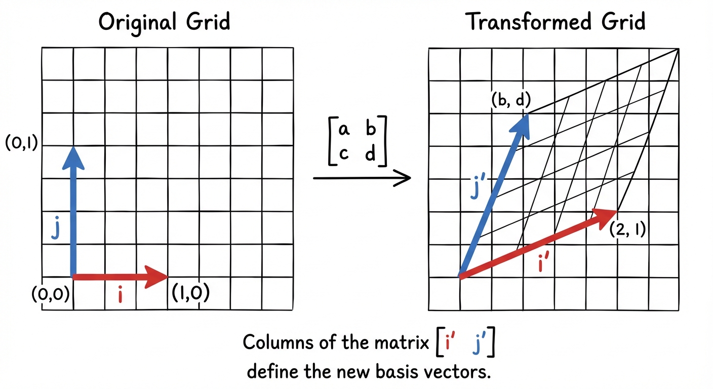
To construct a transformation matrix, figure out where the unit vectors $\mathbf{i} = \langle 1, 0 \rangle$ and $\mathbf{j} = \langle 0, 1 \rangle$ go.
- Column 1 of matrix $M$ is the new position of $\mathbf{i}$.
- Column 2 of matrix $M$ is the new position of $\mathbf{j}$.
4.13 Matrices as Functions
Composition of Functions
If Matrix $A$ represents transformation $f$, and Matrix $B$ represents transformation $g$:
- The transformation $f(g(\mathbf{v}))$ (applying $g$ first, then $f$) is represented by the matrix product $A \cdot B$.
- Order Matters: Since matrix multiplication is not commutative ($AB \neq BA$), the order of transformations matters. The transformation applied first is the matrix on the right.
Inverse Transformations
If a transformation scales and rotates a vector, the inverse matrix reverses that process, returning the vector to its original state.
4.14 Matrices Modeling Contexts
Transition Matrices (Markov Chains)
Matrices are powerful tools for modeling states changing over time (e.g., population migration, customer retention).
- State Vector ($S_0$): A column matrix representing the initial populations or proportions.
- Transition Matrix ($T$): Contains the probabilities or rates of moving from state $j$ (columns) to state $i$ (rows).
Equation for Next State:
To find the state after $k$ steps:
Common Mistakes & Pitfalls
- Order of Matrix Multiplication: Students often multiply $Sn \times T$. This is usually dimensionally impossible. It must be $T \times Sn$ (Matrix $\times$ Vector).
- Calculator Mode: When working with parametric equations involving trig (Circles/Ellipses), ensure your calculator is in Radian mode unless specified otherwise.
- Vector Brackets: Do not use parentheses $(a, b)$ for vectors; use chevrons $\langle a, b \rangle$ to distinguish them from points.
- Inverse Elements: In the inverse formula, students often forget to negate $b$ and $c$, or they swap them instead of swapping $a$ and $d$.
- Determinant Calculation: A common error is calculating $ad + bc$ instead of $ad - bc$.