AP Calculus BC Unit 6 Guidelines: Integration and Accumulation
Approximating Area with Riemann Sums
Before we can calculate the exact area under a curve, we must understand how to approximate it. Calculus uses the concept of accumulation—adding up infinitesimal changes to find a total.
The Geometry of Approximation
A definite integral $\int_a^b f(x) dx$ represents the net signed area between the function $f(x)$ and the x-axis from $x=a$ to $x=b$. We approximate this area using geometric shapes, typically rectangles (Riemann Sums) or trapezoids.
Types of Riemann Sums
Given a partition of the interval $[a, b]$ into $n$ sub-intervals of width $\Delta x$:
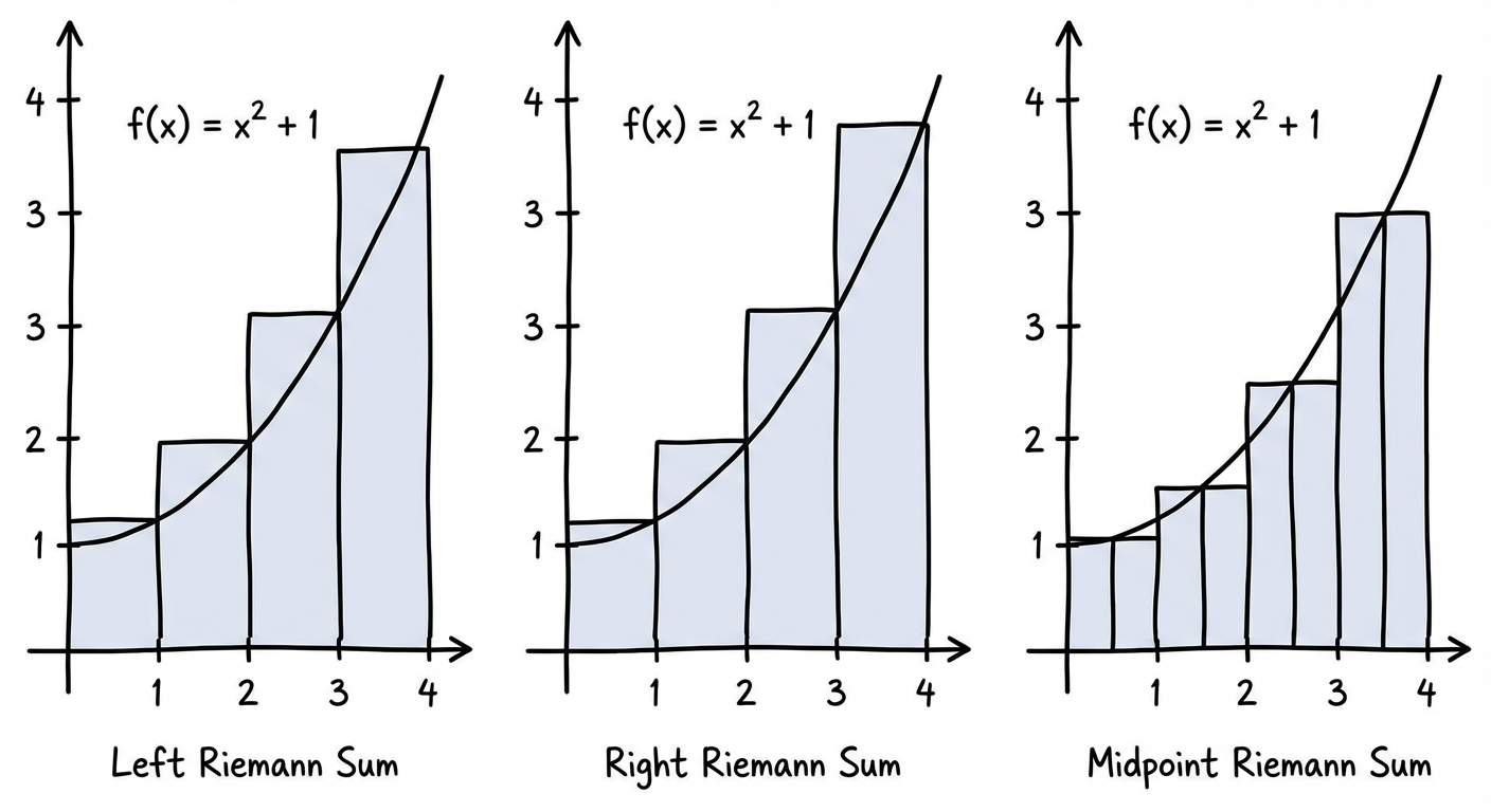
- Left Riemann Sum (LRAM): Uses the height of the function at the left endpoint of each sub-interval.
- Right Riemann Sum (RRAM): Uses the height at the right endpoint.
- Midpoint Riemann Sum (MRAM): Uses the height at the midpoint of the sub-interval.
Key Concept (Over/Under Estimation):
- Increasing Functions: LRAM is an underestimate; RRAM is an overestimate.
- Decreasing Functions: LRAM is an overestimate; RRAM is an underestimate.
- Note: Concavity generally determines errors for Trapezoidal sums, not rectangular sums.
Trapezoidal Sums
A more accurate approximation often uses trapezoids rather than rectangles.
Where $h$ is the width of the interval ($\Delta x$), and $b1, b2$ are the function values ($y$-values) at the endpoints.
Concavity Rule:
- Concave Up: Trapezoidal sum is an overestimate (secant lines lie above curve).
- Concave Down: Trapezoidal sum is an underestimate (secant lines lie below curve).
Tabular Data Problems
On the AP Exam, you are frequently given a table of values rather than a function.
Example: Calculating Approximations
| $t$ (seconds) | 0 | 2 | 5 | 9 |
|---|---|---|---|---|
| $v(t)$ (m/s) | 10 | 18 | 25 | 30 |
Find the Left Riemann Sum and Trapezoidal Sum for $\int_0^9 v(t) dt$.
Solution:
Note that interval widths ($\,\Delta t, $) are not uniform: $2-0=2$, $5-2=3$, $9-5=4$.
1. Left Sum:
(Uses left endpoint $v(t)$ for height)
2. Trapezoidal Sum:
The Definition of the Definite Integral
We move from approximation to exactness using limits. The definite integral is defined as the limit of a Riemann sum as the number of rectangles ($n$) goes to infinity and the width ($\Delta x$) goes to zero.
Where $\Delta x = \frac{b-a}{n}$ and $c_i = a + i\Delta x$ (usually using the right endpoint).
AP Exam Tip: You must be able to recognize a limit in summation form and convert it to an integral.
- Looking for $\frac{b-a}{n}$ (which becomes $dx$)
- Look for the function $f(a + i\frac{b-a}{n})$ (which becomes $f(x)$)
The Fundamental Theorem of Calculus (FTC)
This theorem connects differential calculus (rates of change) with integral calculus (accumulation). It has two parts.
FTC Part 1: The Evaluation Theorem
If $f$ is continuous on $[a, b]$ and $F$ is an antiderivative of $f$:
This calculates the total change of the quantity $F$ over the interval.
Example:
FTC Part 2: Accumulation Functions
This part deals with functions defined by integrals. If $g(x) = \int_a^x f(t) dt$, then:
However, if the upper limit is a function $u(x)$ rather than just $x$, you must apply the Chain Rule:
Worked Problem:
Find $h'(x)$ if $h(x) = \int_2^{x^3} \sin(t^2) dt$.
Solution:
Basic Integration Rules & Properties
Properties of Definite Integrals
- Zero Width: $\int_a^a f(x) dx = 0$
- Reversal: $\inta^b f(x) dx = -\intb^a f(x) dx$
- Additivity: $\inta^c f(x) dx + \intc^b f(x) dx = \int_a^b f(x) dx$
- Linearity: $\int (kf(x) \pm g(x)) dx = k\int f(x)dx \pm \int g(x)dx$
Common Indefinite Integrals
Remember to add $+C$ for indefinite integrals!
| Function | Primitive / Antiderivative |
|---|---|
| $x^n$ | $\frac{x^{n+1}}{n+1} + C$ (Power Rule, $n \neq -1$) |
| $x^{-1}$ or $\frac{1}{x}$ | $\ln |
| $e^x$ | $e^x + C$ |
| $\sin x$ | $-\cos x + C$ |
| $\cos x$ | $\sin x + C$ |
| $\sec^2 x$ | $\tan x + C$ |
| $\frac{1}{1+x^2}$ | $\arctan x + C$ |
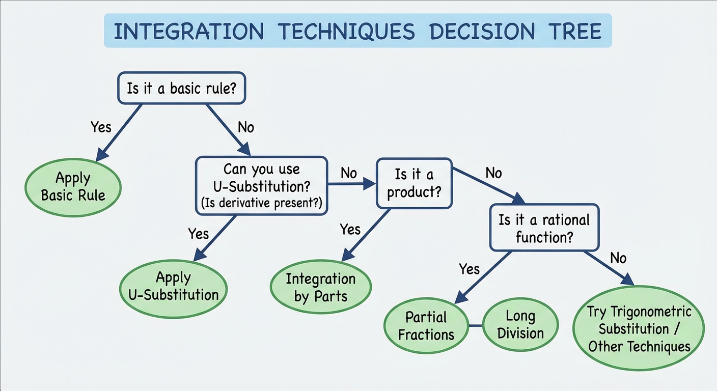
Integration Techniques (AB & BC)
U-Substitution
Used to reverse the Chain Rule. Use when you see a composite function where the derivative of the "inner" part is effectively present elsewhere in the integral.
Algorithm:
- Choose $u$ (usually the inside function).
- Find $du/dx$ and isolate $dx$.
- Critical for Definite Integrals: Change the bounds from $x$-values to $u$-values using your $u$-equation.
- Substitute and integrate.
Example: $\int_0^1 2x(x^2+1)^3 dx$
- Let $u = x^2 + 1$.
- $du = 2x dx \Rightarrow dx = \frac{du}{2x}$.
- Change Bounds:
- If $x=0$, $u = 0^2+1 = 1$.
- If $x=1$, $u = 1^2+1 = 2$.
- Substitute: $\int1^2 2x(u)^3 \frac{du}{2x} = \int1^2 u^3 du$
- Integrate: $[\frac{u^4}{4}]_1^2 = \frac{16}{4} - \frac{1}{4} = \frac{15}{4}$.
Algebraic Manipulation
Before integrating, check if you can simplify using algebra, such as Long Division (usually when degree of numerator $\ge$ degree of denominator) or Completing the Square.
Example (Long Division):
$\int \frac{x^2}{x+1} dx \rightarrow$ Divide $x^2$ by $x+1$ to get $x - 1 + \frac{1}{x+1}$.
Then integrate term by term: $\frac{x^2}{2} - x + \ln|x+1| + C$.
BC Specific Techniques
The following are specific to the AP Calculus BC curriculum and are generally not tested in AB.
Integration by Parts
This is the reverse of the Product Rule. Formula:
Strategy (LIPET):
Order of priority for choosing $u$ (from highest to lowest):
- Logs ($\ln x$)
- Inverse Trig ($\arctan x$)
- Polynomials ($x^2, 3x$)
- Exponentials ($e^x$)
- Trig ($\sin x$)
Integration by Partial Fractions
Used for rational functions where the denominator factors into linear (non-repeating) terms.
Example: Evaluate $\int \frac{1}{x^2 - 5x + 6} dx$
- Factor denominator: $(x-2)(x-3)$.
- Decompose: $\frac{1}{(x-2)(x-3)} = \frac{A}{x-2} + \frac{B}{x-3}$.
- Solve for A and B (Answer: $A=-1, B=1$).
- Integrate: $\int (\frac{-1}{x-2} + \frac{1}{x-3}) dx = -\ln|x-2| + \ln|x-3| + C = \ln|\frac{x-3}{x-2}| + C$.
Improper Integrals
Integrals with efficient bounds or discontinuities.
- Infinite Bounds: Replace $\infty$ with $b$ and take $\lim_{b \to \infty}$.
- Vertical Asymptotes: If the function is undefined at a bound (e.g., $\int0^1 \frac{1}{x} dx$), replace 0 with $a$ and take $\lim{a \to 0^+}$.
Convergence vs. Divergence:
- If the limit exists and is finite, the integral converges.
- If the limit is $\pm \infty$ or DNE, it diverges.
Common Mistakes & Pitfalls
- Forgetting +C: The "classic" calculus mistake. If there are no bounds, you must add the Constant of Integration.
- FTC Part 2 Chain Rule: When differentiating $\int_a^{x^3} f(t)dt$, students forget to multiply by the derivative of the upper bound ($3x^2$).
- Not Changing Bounds in U-Sub: If you switch to $u$, you must calculate new $u$-bounds. Do NOT plug $x$-bounds into a $u$-integral.
- Misinterpreting Area Below X-Axis: Remember definite integrals give net signed area. Area below the axis is negative. Total Area $\neq$ Net Area.
- Trapezoid Rule Formula: Students often forget that the interior terms are multiplied by 2, but the first and last are not. Or they assume width is constant in table problems when it often varies.
- Confusing Average Value with Average Rate of Change:
- Avg Value of function $f$: $\frac{1}{b-a}\int_a^b f(x) dx$
- Avg Rate of Change of $f$: $\frac{f(b)-f(a)}{b-a}$